Computational Physics
A Practical Introduction to Computational
Physics and Scientific Computing (using C++)
Konstantinos N. Anagnostopoulos
National Technical University of Athens
COMPUTATIONAL PHYSICS
A Practical Introduction to Computational Physics and Scientific Computing (C++ version)
AUTHORED BY KONSTANTINOS N. ANAGNOSTOPOULOS
Physics Department, National Technical University of Athens, Zografou Campus, 15780 Zografou,
Greece
konstant@mail.ntua.gr, www.physics.ntua.gr/~konstant/
PUBLISHED BY KONSTANTINOS N. ANAGNOSTOPOULOS
and the
NATIONAL TECHNICAL UNIVERSITY OF ATHENS
Book Website:
www.physics.ntua.gr/~konstant/ComputationalPhysics
©Konstantinos N. Anagnostopoulos 2014, 2016
First Published 2014
Second Edition 2016
Version
2.0.20161206202800
Cover: Design by K.N. Anagnostopoulos. The front cover picture is a snapshot taken during Monte Carlo
simulations of hexatic membranes. Work done with Mark J. Bowick. Relevant video at youtu.be/Erc7Q6YXfLk
 This book and its cover(s) are subject to copyright. They are licensed under the Creative Commons
Attribution-ShareAlike 4.0 International License. To view a copy of this license, visit
creativecommons.org/licenses/by-sa/4.0/
The book is accompanied by software available at the book’s website. All the software, unless the copyright does
not belong to the author, is open source, covered by the GNU public license, see www.gnu.org/licenses/. This is
explicitly mentioned at the end of the respective source files.
ISBN 978-1-365-58322-3 (lulu.com, vol. I)
ISBN 978-1-365-58338-4 (lulu.com, vol. II)
Contents
This book has been written assuming that the reader executes all
the commands presented in the text and follows all the
instructions at the same time. If this advice is neglected, then
the book will be of little help and some parts of the text may seem
incomprehensible.
The book’s website is at
http://www.physics.ntua.gr/~konstant/ComputationalPhysics/
From there, you can can download the accompanying software, which
contains, among other things, all the programs presented in the book.
Some conventions: Text using the font shown below refers to commands
given using a shell (the “command line”), input and output of programs, code
written in Fortran (or any other programming language), as well as to names of
files and programs:
> echo Hello world
Hello world
When a line starts with the prompt
>
then the text that follows is a command, which can be given from the command
line of a terminal. The second line, Hello World, is the output of the
command.
The contents of a file with C++ code is listed below:
int main(){
double x = 0.0;
for(int i=0;i<10;i++){
x += i;
}
}
What you need in order to work on your PC:
- An operating system of the GNU/Linux family and its basic tools.
- A Fortran compiler. The gfortran compiler is freely available
for all major operating systems under an open source license at
http://www.gfortran.org.
- An advanced text editor, suitable for editing code in several programming
languages, like Emacs .
- A good plotting program, suitable for data analysis, like gnuplot .
- The shell tcsh .
- The programs awk ,
grep, sort, cat, head, tail, less. Make sure that they are available
in your computer environment.
If you have installed a GNU/Linux distribution on your computer, all of the
above can be installed easily. For example, in a Debian like distribution (Ubuntu,
...) the commands
> sudo apt-get install tcsh emacs gnuplot gnuplot-doc
> sudo apt-get install gfortran gawk gawk-doc binutils
> sudo apt-get install manpages-dev coreutils liblapack3
install all the necessary tools.
If you don’t wish to install GNU/Linux on your computer, you can try the
following:
- Boot your computer using a usb/DVD live GNU/Linux, like Ubuntu .
This will not make any permanent changes in your hard drive but it
will start and run slower. On the other hand, you may save all your
computing environment and documents and use it on any computer
you like.
- Install Cygwin
in your Microsoft Windows. It is a very good solution for Microsoft-addicted
users. If you choose the full installation, then you will find all the tools
needed in this book.
- Mac OS X is based on Unix. It is possible to install all the software
needed in this book and follow the material as presented. Search the
internet for instructions, e.g. google “gfortran for Mac”, “emacs for
Mac”, “tcsh for Mac”, etc.
Foreword to the Second Edition
This book has been out “in the wild” for more than two years. Since then, its pdf
version has been downloaded 2-5000 times/month from the main server and has a
few thousand hits from sites that offer science e-books for free. I have also
received positive feedback from students and colleagues from all over
the world and that gave me the encouragement to devote some time to
create a C++ version of the book. As far as scientific programming is
concerned, the material has not changed apart from some typo and error
corrections .
I have to make it clear that by using this book you will not learn much on the
advanced features of C++. Scientific computing is usually simple at its core
and, since it must be made efficient and accurate, it needs to go down
to the lowest levels of programming. This also partly the reason of why
I chose to use Fortran for the core programming in the first edition of
the book: It is a language designed for numerical programming and high
performance computing in mind. It is simple and a scientist or engineer can go
directly into programming her code. C++ is not designed for scientific
applications
in mind and this reflects on some trivial omissions in its standard. Still, many
scientific groups are now using C++ for programming and the C++ compilers
have improved quite a lot. There is still an advantage in performance using a
Fortran compiler on a supercomputer, but this is not going to last for much
longer.
Still, for a scientist, the programming language is a tool to solve her scientific
problems. One should not bind herself to a specific language. The treasures of
today are the garbage of tomorrow, and the time scale for this happening is small
in today’s computing environments. What has really lasting value is the
ability to solve problems using a computer and this is what needs to be
emphasized. Consistent with this idea is that, in the course of reading this
book, you will also learn how to make your C++ code interact with code
written in Fortran, like in the case of the popular library Lapack. This will
improve your “multilingual skills” and flexibility with interacting with legacy
code.
The good news for us scientists is that numerical code usually needs simple
data structures and programming is similar in any language. It was simple for
me to “translate” my book from Fortran to C++. Unfortunately I will
not touch on all this great stuff in true object oriented programming
but you may be happy to know that you will most likely not need
it .
So, I hope that you will enjoy using my book and I remind you that I love fan
mail and I appreciate comments/corrections/suggestions sent to me. Now, if you
want to learn about the structure and educational procedure in this book, read
the foreword to the first edition, otherwise skip to the real fun of solving scientific
problems numerically.
Athens, 2016.
Foreword to the First Edition
This book is the culmination of my ten years’ experience in teaching three
introductory, undergraduate level, scientific computing/computational physics
classes at the National Technical University of Athens. It is suitable mostly
for junior or senior level science courses, but I am currently teaching its
first chapters to sophomores without a problem. A two semester course
can easily cover all the material in the book, including lab sessions for
practicing.
Why another book in computational physics? Well, when I started teaching
those classes there was no bibliography available in Greek, so I was compelled to
write lecture notes for my students. Soon, I realized that my students, majoring in
physics or applied mathematics, were having a hard time with the technical
details of programming and computing, rather than with the physics concepts. I
had to take them slowly by the hand through the “howto” of computing,
something that is reflected in the philosophy of this book. Hoping that this could
be useful to a wider audience, I decided to translate these notes in English
and put them in an order and structure that would turn them into “a
book”.
I also decided to make the book freely available on the web. I was
partly motivated by my anger caused by the increase of academic (e)book
prices to ridiculous levels during times of plummeting publishing costs.
Publishers play a diminishing role in academic publishing. They get an almost
ready-made manuscript in electronic form by the author. They need to
take no serious investment risk on an edition, thanks to print-on-demand
capabilities. They have virtually zero cost ebook publishing. Moreover, online
bookstores have decreased costs quite a lot. Academic books need no
advertisement budget, their success is due to their academic reputation. I don’t
see all of these reflected on reduced book prices, quite the contrary, I’m
afraid.
My main motivation, however, is the freedom that independent publishing
would give me in improving, expanding and changing the book in the future. It is
great to have no length restrictions for the presentation of the material, as well as
not having to report to a publisher. The reader/instructor that finds the book
long, can read/print the portion of the book that she finds useful for
her.
This is not a reference book. It uses some interesting, I hope, physics problems
in order to introduce the student to the fundamentals of solving a scientific
problem numerically. At the same time, it keeps an eye in the direction of
advanced and high performance scientific computing. The reader should follow the
instructions given in each chapter, since the book teaches by example. Several
skills are taught through the solution of a particular problem. My lectures take
place in a (large) computer lab, where the students are simultaneously doing
what I am doing (and more). The program that I am editing and the
commands that I am executing are shown on a large screen, displaying my
computer monitor and actions live. The book provides no systematic
teaching of a programming language or a particular tool. A very basic
introduction is given in the first chapter and then the reader learns whatever is
necessary for the solution of her problem. There is more than one way to do
it
and the problems can be solved by following a basic or a fancy way, depending on
the student’s computational literacy. The book provides the necessary tools for
both. A bibliography is provided at the end of the book, so that the missing pieces
of a puzzle can be sought in the literature.
This is also not a computational physics playground. Of course I hope that the
reader will have fun doing what is in the book, but my goal is to provide an
experience that will set the solid foundation for her becoming a high performance
computing, number crunching, heavy duty data analysis expert in the future. This
is why the programming language of the core numerical algorithms has
been chosen to be Fortran, a highly optimized, scientifically oriented,
programming language. The computer environment is set in a Unix family
operating system, enriched by all the powerful GNU tools provided by the
FSF .
These tools are indispensable in the complicated data manipulation needed in
scientific research, which requires flexibility and imagination. Of course,
Fortran is not the best choice for heavy duty object oriented programming,
and is not optimal for interacting with the operating system. The
philosophy
is to let Fortran do what is best for, number crunching, and leave data
manipulation and file administration to external, powerful tools. Tools, like
awk, shell scripting, gnuplot, Perl and others, are quite powerful and
complement all the weaknesses of Fortran mentioned before. The plotting
program is chosen to be gnuplot, which provides very powerful tools to
manipulate the data and create massive and complicated plots. It can
also create publication quality plots and contribute to the “fun part” of
the learning experience by creating animations, interactive 3d plots etc.
All the tools used in the book are open source software and they are
accessible to everyone for free. They can be used in a Linux environment, but
they can also be installed and used in Microsoft Windows and Mac OS
X.
The other hard part in teaching computational physics to scientists and
engineers is to explain that the approach of solving a problem numerically is quite
different from solving it analytically. Usually, students of this level are coming
with a background in analysis and fundamental physics. It is hard to
put them into the mode of thinking about solving a problem using only
additions, multiplications and some logical operations. The hardest part is to
explain the discretization of a model defined analytically, which can be done
in many ways, depending on the accuracy of the approximation. Then,
one has to extrapolate the numerical solution, in order to obtain a good
approximation of the analytic one. This is done step by step in the book, starting
with problems in simple motion and ending with discussing finite size
scaling in statistical physics models in the vicinity of a continuous phase
transition.
The book comes together with additional material which can be found at the web page
of the book .
The accompanying software contains all the computer programs presented in the
book, together with useful tools and programs solving some of the exercises of
each chapter. Each chapter has problems complementing the material
covered in the text. The student needs to solve them in order to obtain
hands on experience in scientific computing. I hope that I have already
stressed enough that, in order for this book to be useful, it is not enough
to be read in a café or in a living room, but one needs to do what it
says.
Hoping that this book will be useful to you as a student or as an instructor, I
would like to ask you to take some time to send me feedback for improving and/or
correcting it. I would also appreciate fan mail or, if you are an expert, a review of
the book. If you use the book in a class, as a main textbook or as supplementary
material, I would also be thrilled to know about it. Send me email at
konstantmail.ntua.gr and let me know if I can publish, anonymously or not,
(part of) what you say on the web page (otherwise I will only use it privately
for my personal ego-boost). Well, nothing is given for free: As one of
my friends says, some people are payed in dollars and some others in
ego-dollars!
Have fun computing scientifically!
Athens, 2014.
Chapter 1
The Computer
The aim of this chapter is to lay the grounds for the development of the
computational skills which are necessary in the following chapters. It is not an in
depth exposition but a practical training by example. For a more systematic study
of the topics discussed, we refer to the bibliography. Many of the references are
freely available n the web.
The are many choices that one has to make when designing a computer
project. These depend on the needs for numerical efficiency, on available
programming hours, on the needs for extensibility and upgradability and so on. In
this book we will get the flavor of a project that is mostly scientifically and
number crunching oriented. One has to make the best of the available computing
resources and have powerful tools available for a productive analysis of the data.
Such an environment, found in most of today’s supercomputers, that offers
flexibility, dependability, simplicity, powerful tools for data analysis and effective
compilers is provided by the family of the Unix operating systems. The
GNU/Linux operating system is a Unix variant that is freely available
and most of its utilities are open source software. The voluntary work of
millions of excellent programmers worldwide has built the most stable,
fastest and highest quality software available for scientific computing today.
Thanks to the idea of the open source software pioneered by Richard
Stallman
this giant collaboration has been made possible.
Another choice that we have to make is the programming language.
In this edition of the book we will be programming in C++. C++ is a
language with very high level of abstraction designed for projects where
modular programming and the use of complicated data structures is of very
high priority. A large and complicated project should be divided into
independent programming tasks (modules), where each task contains
everything that it needs and does not interfere with the functionality of
other modules. Although it has not been designed for high performance
numerical applications, it is becoming more and more popular in the recent
years.
C++, as well as other languages like C, Java and Fortran, is a language that
needs to be compiled by a compiler. Other languages, like python, perl, awk, shell
scripting, Macsyma, Mathematica, Octave, Matlab,  , are interpreted
line by line. These languages can be simple in their use, but they can be
prohibitively slow when it comes to a numerically demanding program. A
compiler is a tool that analyzes the whole program and optimizes the
computer instructions executed by the computer. But if programming time is
more valuable, then a simple, interpreted language can lead to faster
results.
Another choice that we make in this book, and we mention it because it is not the
default in most Linux distributions, is the choice of shell. The shell is a program that
“connects” the user to the operating system. In this book, we will teach how to use a
shell
to “send” commands to the operating system, which is the most effective way to
perform complicated tasks. We will use the shell tcsh, although most of the
commands can be interpreted by most popular shells. Shell scripting is simpler in
this shell, although shells like bash provide more powerful tools, mostly needed
for complicated system administration tasks. That may cause a small
inconvenience to some readers, since tcsh is not preinstalled in Linux
distributions .
1.1 The Operating System
The Unix family of operating systems offer an environment where complicated
tasks can be accomplished by combining many different tools, each of which
performs a distinct task. This way, one can use the power of each tool, so that
trivial but complicated parts of a calculation don’t have to be programmed. This
makes the life of a researcher much easier and much more productive, since
research requires from us to try many things before we understand how to
compute what we are looking for.
In the Unix operating system everything is a file, and files are organized in a
unique and unified filesystem. Documents, pictures, music, movies, executable
programs are files. But also directories or devices, like hard disks, monitors, mice,
sound cards etc, are, from the point of view of the operating system, files. In order
for a music file to be played by your computer, the music data needs to be written
to a device file, connected by the operating system to the sound card. The
characters you type in a terminal are read from a file “the keyboard”,
and written to a file “the monitor” in order to be displayed. Therefore,
the first thing that we need to understand is the structure of the Unix
filesystem.
1.1.1 Filesystem
There is at least one path in the filesystem associated with each file. There
are two types of paths, relative paths and absolute paths. These are two
examples:
bin/RungeKutta/rk.exe
/home/george/bin/RungeKutta/rk.exe
The paths shown above may refer to the same or a different file. This
depends on “where we are”. If “we are” in the directory /home/george,
then both paths refer to the same file. If on the other way “we are” in a
directory /home/john or /home/george/CompPhys, then the paths
refer
to two different files. In the last two cases, the paths refer to the files
/home/john/bin/RungeKutta/rk.exe
/home/george/CompPhys/bin/RungeKutta/rk.exe
respectively. How can we tell the difference? An absolute path always begins with
the / character, whereas a relative path does not. When we say that “we are in a
directory”, we refer to a position in the filesystem called the current directory, or
working directory. Every process in the operating system has a unique current
directory associated with it.
The filesystem is built on its root and looks like a tree positioned upside down.
The symbol of the root is the character / The root is a directory. Every directory
is a file that contains a list of files, and it is connected to a unique directory, its
parent directory . Its list of files contains other directories, called its subdirectories,
which all have it as their parent directory. All these files are the contents
of the directory. Therefore, the filesystem is a tree of directories with
the root directory at its top which branch to its subdirectories, which in
their turn branch into other subdirectories and so on. There is practically
no limit to how large this tree can become, even for a quite demanding
environment .
A path consists of a string of characters, with the characters / separating its
components, and refers to a unique location in the filesystem. Every component
refers to a file. All, but the last one, must be directories in a hierarchy, from
parent directory to subdirectory. The only exception is a possible / in the
beginning, which refers to the root directory. Such an example can be seen in
figure 1.1.
In a Unix filesystem there is complete freedom in the choice of the location of the
files .
Fortunately, there are some universally accepted conventions respected by almost
everyone. One expects to find home directories in the directory /home,
configuration files in the directory /etc, application executables in directories
with names such as /bin, /usr/bin, /usr/local/bin, software libraries in
directories with names such as /lib, /usr/lib etc.
There are some important conventions in the naming of the paths. A single
dot “.” refers to the current directory and a double dot “..” to the parent
directory. Similarly, a tilde “~” refers to the home directory of the user. Assume,
e.g., that we are the user george running a process with a current directory
/home/george/Music/Rock (see figure 1.1). Then, the following paths refer to the
same file /home/george/Doc/lyrics.doc:
../../Doc/lyrics.doc
~/Doc/lyrics.doc
~george/Doc/lyrics.doc
./../../Doc/lyrics.doc
Notice that ~ and ~george refer to the home directory of the user george
(ourselves), whereas ~mary refer to the home directory of another user,
mary.
We are now going to introduce the basic commands for filesystem navigation and
manipulation .
The command cd (=change directory) changes the current directory, whereas the
command pwd (=print working directory) prints the current directory:
> cd /usr/bin
> pwd
/usr/bin
> cd /usr/local/lib
> pwd
/usr/local/lib
> cd
> pwd
/home/george
> cd -
> pwd
/usr/local/lib
> cd ../../
> pwd
/usr
The argument of the command cd is an absolute or a relative path. If the path is
correct and we have the necessary permissions, the command changes the current
directory to this path. If no path is given, then the current directory changes to
the home directory of the user. If the character - is given instead of a path,
then the command changes the current directory to the previous current
directory.
The command mkdir creates new directories, whereas the command rmdir
removes empty directories. Try:
> mkdir new
> mkdir new/01
> mkdir new/01/02/03
mkdir: cannot create directory ‘new/01/02/03’: No such file or
directory
> mkdir -p new/01/02/03
> rmdir new
rmdir: ‘new’: Directory not empty
> rmdir new/01/02/03
> rmdir new/01/02
> rmdir new/01
> rmdir new
Note that the command mkdir cannot create directories more than one level
down the filesystem, whereas the command mkdir -p can. The “switch” -p makes
the behavior of the command different than the default one.
In order to list the contents of a directory, we use the command ls
(=list):
> ls
BE.eps Byz.eps Programs srBE_xyz.eps srB_xyz.eps
B.eps Bzy.eps srBd_xyz.eps srB_xy.eps
> ls Programs
Backup rk3_Byz.cpp rk3.cpp
plot-commands rk3_Bz.cpp rk3_g.cpp
The first command is given without an argument and it lists the contents of the
current directory. The second one, lists the contents of the subdirectory of the
current directory Programs. If the argument is a list of paths pointing to regular
files, then the command prints the names of the paths. Another way of giving the
command is
[literate={-}{{\texttt{-}}}1]%[basicstyle=\ttfamily]
> ls -l
total 252
-rw-r--r-- 1 george users 24284 May 1 12:08 BE.eps
-rw-r--r-- 1 george users 22024 May 1 11:53 B.eps
-rw-r--r-- 1 george users 29935 May 1 13:02 Byz.eps
-rw-r--r-- 1 george users 48708 May 1 12:41 Bzy.eps
drwxr-xr-x 4 george users 4096 May 1 23:38 Programs
-rw-r--r-- 1 george users 41224 May 1 22:56 srBd_xyz.eps
-rw-r--r-- 1 george users 23187 May 1 21:13 srBE_xyz.eps
-rw-r--r-- 1 george users 24610 May 1 20:29 srB_xy.eps
-rw-r--r-- 1 george users 23763 May 1 20:29 srB_xyz.eps
The switch -l makes ls to list the contents of the current directory together with
useful information on the files in 9 columns. The first column lists the permissions
of the files (see below). The second one lists the number of links of the
files .
The third one lists the user who is the owner of each file. The fourth one lists the
group that is assigned to the files. The fifth one lists the size of the file in bytes
(=8 bits). The next three ones list the modification time of the file and the last
one the paths of the files.
File permissions
are separated in three classes: owner permissions, group permissions and other
permissions. Each class is given three specific permissions, r=read, w=write and
x=execute. For regular files, read permission effectively means access to the file
for reading/copying, write permission means permission to modify the contents of
the file and execute permission means permission to execute the file as a
command .
For directories, read permission means that one is able to read the names of the
files in the directory (but not make it as current directory with the cd command),
write permission means to be able to modify its contents (i.e. create, delete, and
rename files) and execute permission grants permission to access/modify the
contents of the files (but not list the names of the files, this is granted by the read
permission).
The command ls -l lists permissions in three groups. The owner (positions
2-4), the group (positions 5-7) and the rest of the world (others - positions 8-10).
For example
[literate={-}{{\texttt{-}}}1]
-rw-r--r--
-rwxr-----
drwx--x--x
In the first case, the owner has read and write but not execute permissions and
the group+others have only read permissions. In the second case, the user has
read, write and execute permissions, the group has read permissions and others
have no permissions at all. In the last case, the user has read, write and execute
permissions, whereas the group and the world have only execute permissions. The
first character d indicates a special file, which in this case is a directory. All
special files have this position set to a character, while regular files have it set to
-.
File permissions can be modified by using the command chmod:
> chmod u+x file
> chmod og-w file1 file2
> chmod a+r file
Using the first command, the owner (u user) obtains (+) permission to
execute (x) the file named file. Using the second one, the rest of the world (o
 others) and the group (g
 group) loose (-) the write (w) permission to the files
named file1 and file2. Using the third one, everyone (a
 all) obtain read (r)
permission on the file named file.
We will close this section by discussing some commands which are used for
administering files in the filesystem. The command cp (copy) copies the contents
of files into other files:
> cp file1.cpp file2.cpp
> cp file1.cpp file2.cpp file3.cpp Programs
If the file file2.cpp does not exist, the first command copies the contents of
file1.cpp to a new file file2.cpp. If it already exists, it replaces its
contents by the contents of the file file2.cpp. In order for the second
command to be executed, Programs needs to be a directory. Then, the
contents of the files file1.cpp, file2.cpp, file3.cpp are copied to
indentical files in the directory Programs. Of course, we assume that
the user has the appropriate privileges for the command to be executed
successfully.
The command mv “moves”, or renames, files:
> mv file1.cpp file2.cpp
> mv file1.cpp file2.cpp file3.cpp Programs
The first command renames the file file1.cpp to file2.cpp. The second
one moves files file1.cpp, file2.cpp, file3.cpp into the directory
Programs.
The command rm (remove) deletes
files .
Beware, the command is unforgiving: after deletion, a file cannot be restored into the
filesystem .
Therefore, after executing successfully the following commands
> ls
file1.cpp file2.cpp file3.cpp file4.csh
> rm file1.cpp file2.cpp file3.cpp
> ls
file4.csh
the files file1.cpp, file2.cpp, file3.cpp do not exist in the filesystem
anymore. A more prudent use of the command demands the flag -i. Then, before
deletion we are asked for confirmation:
> rm -i *
rm: remove regular file ‘file1.cpp’? y
rm: remove regular file ‘file2.cpp’? y
rm: remove regular file ‘file3.cpp’? y
rm: remove regular file ‘file4.csh’? n
> ls
file4.csh
When we type y, the file is deleted, when we type n, the file is not deleted.
We cannot remove directories the same way. It is possible to use the command
rmdir in order to remove empty directories. In order to delete directories together
with their contents (including subdirectories and their contents) use the
command
rm -r. For example, assume that the contents of the directories dir1 and
dir1/dir2 are the files:
./dir1
./dir1/file2.cpp
./dir1/file1.cpp
./dir1/dir2
./dir1/dir2/file3.cpp
Then the results of the following commands are:
> rm dir1
rm: cannot remove ‘dir1’: Is a directory
> rm dir1/dir2
rm: cannot remove ‘dir1/dir2’: Is a directory
> rmdir dir1
rmdir: dir1: Directory not empty
> rmdir dir1/dir2
rmdir: dir1/dir2: Directory not empty
> rm -r dir1
The last command removes all files (assuming that we have write permissions
for all directories and subdirectories). Alternatively, we can empty the
contents of all directories first, and then remove them with the command
rmdir:
> cd dir1/dir2; rm file3.cpp
> cd .. ; rmdir dir2
> rm file1.cpp file2.cpp
> cd .. ; rmdir dir1
Note that by using a semicolon, we can execute two or more commands on the
same line.
1.1.2 Commands
Commands in a Unix operating system are files with execute permission. When
we write a sentence on the command line, like
> ls -l test.cpp test.dat
the shell reads its and interprets it. The shell is a program that creates a interface
between a user and the operating system. The first word (ls) of the sentence is
interpreted as a command. The rest of the words are the arguments of the
command and the program can use them (or not) at the discretion of its
programmer. There is a special convention for arguments that begin with a - (e.g.
-l, --help, --version, -O3). They are called options or switches, and they act as
virtual switches that make the program act in a particular way. We have
already seen that the program ls gives a different output with the switch
-l.
In order for a command to be executed, the shell looks for a file that has the
same name as the command (here a file named ls). In order to understand where
the shell looks for such a file, we should digress a little bit and explain the use
of shell variables and environment variables. These have a name, which
is a string of permissible characters, and their values are obtained by
preceding their name with the $ character. For example the variable PATH has
value $PATH. The values of the environment variables can be set with the
command
setenv and of the shell variables with the command set:
> setenv MYVAR test-env
> set myvar = test-shell
> echo $MYVAR $myvar
test-env test-shell
Two special variables are the variables PATH and path:
>echo $PATH
/usr/local/bin:/usr/bin:/bin:/usr/X11/bin
>echo $path
/usr/local/bin /usr/bin /bin /usr/X11/bin
The first one is an environment variable and the second one is a shell variable.
Their values are set by the shell, and we don’t need to worry about them, unless
we want to change them. Their value is a string of characters whose components
should be valid paths to directories. In the first case, the components are
separated by a :, while in the second case, by one or more spaces. In the
example shown above, the shell searches each component of the path or
PATH variables (in this order) until it finds a file ls in their contents. If
it succeeds and the file has execute permissions, then the program in
this file is executed. If it fails, then it prints an error message. Try the
commands:
> which ls
/bin/ls
> ls -l /bin/ls
-rwxr-xr-x 1 root root 93560 Sep 28 2006 /bin/ls
We see that the program that the ls command executes the program in the file
/bin/ls.
The arguments of a command are passed on to the program that the command
executes for possible interpretation. For example:
> ls -l test.cpp test.dat
The argument -l is the switch that results in a long listing of the files. The
arguments test.cpp and test.dat are interpreted by the program ls as paths
that it will look up for file information.
You can use the * (wildcard) character as a shorthand notation for a group of
files. For example, in the command shown below
> ls -l *.cpp *.dat
the shell will expand *.cpp and *.dat to a list of all files whose names end with
.cpp or .dat. Therefore, if the current directory contains the files test.cpp,
test1.cpp, myprog.cpp, test.dat, hello.dat, the arguments that will be
passed on to the command ls are
> ls -l myprog.cpp test1.cpp test.cpp hello.dat test.dat
For each command there are three special files associated with it. The first
one is the standard input (stdin), the second one is the standard output
(stdout) and the third one the standard error (stderr). These are files
where the program can print or read data from. By default, these files are
the terminal that the user uses to execute the command. In this case,
when the program reads data from the stdin, then it reads the data that
we type to the terminal using the keyboard. When the program writes
data to the stdout or to the stderr, then the data is written to the
terminal.
The advantage of using these special files in order to read/write data is that
the user can redirect the input/output to these files to any file she wants. Using
the character > at the end of a command redirects the stdout to the file whose
name is written after >. For example:
> ls
file1.cpp file2.cpp file3.cpp file4.csh
> ls > results
> ls
file1.cpp file2.cpp file3.cpp file4.csh results
The first of the above commands, prints the contents of the current working
directory to the terminal. The second command redirects data written to
the stdout to the file results. After executing the command, the file
results is created and its contents are the names of the files file1.cpp
file2.cpp file3.cpp file4.csh. If the file results does not exist
(as in the above example), the file is created. If it already exists, it is
truncated and its contents replaced by the data written to the stdout of the
command. If we want to append data without erasing the existing contents,
then we should use the string of characters >>. Therefore, if we give the
command
> ls >> results
after executing the previous commands, then the contents of the file results will
be
file1.cpp file2.cpp file3.cpp file4.csh
file1.cpp file2.cpp file3.cpp file4.csh results
The redirection of the stdin is accomplished by the use of the
character < while that of the stderr by the use of the string of
characters
>&. We will see more examples in section 1.2.
It is possible to redirect the stdout of a command to be the stdin of
another command. This is very useful for creating filters. A filter is a
command that creates a flow of data between two or more programs.
This process is called piping. Pipes are creating by using the character
|
> cmd1 | cmd2 | cmd3 | ... | cmdN
Using the syntax shown above, the stdout of the command cmd1 is redirected to
the stdin of the command cmd2, the stdout of the command cmd2 is redirected
to the stdin of the command cmd3 etc. More examples will be presented in
section 1.2.
1.1.3 Looking for Help
Unix got itself a reputation for not being user friendly. This is far from the truth.
Although there is a steep learning curve, detailed documentation for almost
everything is available online.
The key for a comfortable ride is to learn how to use the help system available
on your computer and on the internet. Most of the commands are self
documented. A simple test, like the one shown below, will help you with the basic
usage of most of the commands:
[literate={-}{{\texttt{-}}}1]
> cmd --help
> cmd -h
> cmd -help
> cmd -\?
For example, try the command ls --help. For a window application, start from
the menu “Help”. You should not be afraid and/or lazy and you should proceed
with careful searching and reading.
For example, let’s assume that you have heard about a command that sounds
like printf, or something like that. The first level of online help is the man
(=manual) command that searches the “man pages”. Read the output of the
command
> man printf
The command info usually provides more detailed and user friendly
documentation. It has basic browsing capabilities like the browsers you use to
read pages from the internet. Try the command
> info printf
Furthermore, the commands
> man -k printf
> whatis printf
will inform you that there are other, possibly related, commands with names like
fprintf, fwprintf, wprintf, sprintf...:
> whatis printf
printf (1) - format and print data
printf (1p) - write formatted output
printf (3) - formatted output conversion
printf (3p) - print formatted output
printf [builtins] (1) - bash built-in commands, see bash(1)
The second column printed by the whatis command is the “section” of the man
pages. In order to gain access to the information in a particular section, you have
to give it as an argument to the man command:
> man 1 printf
> man 1p printf
> man 3 printf
> man 3p printf
> man bash
Section 1 of the man pages contains information of ordinary command line
commands, section 3 contains information on functions in libraries of
the C language. Section 2 contains information on commands used for
system administration. You may browse the directory /usr/share/man, or
read the man page of the man command (use the command man man for
that!).
By using the command
[literate={-}{{\texttt{-}}}1]
> printf --help
we obtain plenty of memory refreshing information. The command
> locate printf
shows us many files related to the command printf. The commands
> which printf
> where printf
give information on the location of the executable(s) of the command
printf.
Another useful feature of the shell is the command or it filename completion.
This means that we can write only the first characters of the name
of a command or filename and then press simultaneously the keys
[Ctrl-d]
(i.e. press the key Ctrl and the key of the letter d at the same time). Then the shell will
complete the name of the command up to the point that is is unique with the given string of
characters :
> pri[Ctrl-d]
printafm printf printenv printnodetest
Try to type an x on the command line and then type [Ctrl-d]. You will learn all
the commands that are available and whose name begins with an x: xterm,
xeyes, xclock, xcalc, ...
Finally, the internet contains a wealth of information. Google your blues... and
you will be rewarded!
1.2 Text Processing Tools – Filters
For doing data analysis, we will need powerful tools for manipulating data in text
files. These are files that consist solely of printable characters. Some tools that can
be used in order to construct complicated and powerful filters are the programs
cat, less, head, tail, grep, sort and awk.
Suppose that we have data in a file named
data
which contains information on the contents of a food warehouse and their
prices:
bananas 100 pieces 1.45
apples 325 boxes 1.18
pears 34 kilos 2.46
bread 62 kilos 0.60
ham 85 kilos 3.56
The command
> cat data
prints the contents of the file data to the stdout. In general, this command
prints the contents of all files given in its arguments or the stdin if none is given.
Since the stdin and the stdout can be redirected, the command
> cat < data > data1
takes the contents of the file data from the stdin and prints them to the stdout,
which in this case is the file data1. This command has the same result as the
command:
> cp data data1
The command
> cat data data1 > data2
prints the contents of the file data and then the contents of the file data1 to the
stdout. Since the stdout is redirected to the file data2, data2 contains the data
of both files.
By giving the command
> less gfortran.txt
you can browse the data contained in the file gfortran.txt one page at a time.
Press [space] in order to “turn” a page, [b] to turn back a page. Press the up
and down arrows to move one line backwards/forward. Press [g] in order to
jump to the beginning of the file and press [G] in order to jump to the
end. Press [h] in order to get a help message and press [q] in order to
quit.
The commands
> head -n 1 data
bananas 100 pieces 1.45
> tail -n 2 data
bread 62 kilos 0.60
ham 85 kilos 3.56
> tail -n 2 data | head -n 1
bread 62 kilos 0.60
print the first line, the last two lines and the second to the last line of the file
data to the stdout respectively. Note that, by piping the stdout of the command
tail to the stdin of the command head, we are able to construct the filter “print
the line before the last one”.
The command sort sorts the contents of a file by comparing each line of its
text with all others. The sorting is alphabetical, unless otherwise set by using
options. For example
> sort data
apples 325 boxes 1.18
bananas 100 pieces 1.45
bread 62 kilos 0.60
ham 85 kilos 3.56
pears 34 kilos 2.46
For reverse sorting, try sort -r data. We can also sort by comparing specific
fields of each line. By default, fields are words separated by one or more spaces.
For example, in order to sort w.r.t. the second column of the file data, we can use
the switch -k 2 (=second field). Furthermore, we can use the switch -n for
numerical sorting:
> sort -k 2 -n data
pears 34 kilos 2.46
bread 62 kilos 0.60
ham 85 kilos 3.56
bananas 100 pieces 1.45
apples 325 boxes 1.18
If we omit the switch -n, the comparison of the lines is performed based on
character sorting of the second field and the result is
> sort -k 2 data
bananas 100 pieces 1.45
apples 325 boxes 1.18
pears 34 kilos 2.46
bread 62 kilos 0.60
ham 85 kilos 3.56
The last column contains floating point numbers (not integers). In order to sort
by the values of such numbers we should use the switch -g:
> sort -k 4 -g data
bread 62 kilos 0.60
apples 325 boxes 1.18
bananas 100 pieces 1.45
pears 34 kilos 2.46
ham 85 kilos 3.56
The command grep processes a text file line by line, searching for a given
string of characters. When this string is found anywhere in a line, this line is
printed to the stdout. The command
> grep kilos data
pears 34 kilos 2.46
bread 62 kilos 0.60
ham 85 kilos 3.56
prints each line containing the string “kilos”. If we want to search for all line not
containing the string “kilos”, then we add the switch -v:
> grep -v kilos data
bananas 100 pieces 1.45
apples 325 boxes 1.18
We can use a regular expression for searching a whole family of strings of
characters. These monsters need a full book for discussing them in detail! But it is
not hard to learn how to use some simple forms of regular expressions. Here are
some examples:
> grep ^b data
bananas 100 pieces 1.45
bread 62 kilos 0.60
> grep ’0$’ data
bread 62 kilos 0.60
> grep ’3[24]’ data
apples 325 boxes 1.18
pears 34 kilos 2.46
The first one, prints each line whose first character is a b. The second one, prints
each line that ends with a 0. The third one, prints each line contaning the strings
32 or 34.
By far, the strongest tool in our toolbox is the awk program. By default, awk
analyzes a text file line by line. Each word (or field in the awk jargon) of these
lines is stored in a set of variables with names $1, $2, .... The variable $0
contains the full line currently processed, whereas the variable NF counts the
number of fields in the current line. The variable NR counts the number of lines of
the file processed so far by awk.
An awk program can be written in the command line. A set of commands
within { ... } is executed for each line of input. The constructs BEGIN{ ... }
and END{ ... } contain commands executed, only once, before and after the
processing of the file respectively. For example, the command
> awk ’{print $1,"total value= ",$2*$4}’ data
bananas total value= 145
apples total value= 383.5
pears total value= 83.64
bread total value= 37.2
ham total value= 302.6
prints the name of the product (1st column = $1) and the total value stored in
the warehouse (2nd column = $2)  (4th column = $4). More examples are
given below:
> awk ’{value += $2*$4}END{print "Total= ",value}’ data
Total= 951.94
> awk ’{av += $4}END{print "Average Price= ",av/NR}’ data
Average Price= 1.85
> awk ’{print $2^2 * sin($4) + exp($4)}’ data
The first one calculates the total value of all products: The processing of each line
results in the increment (+=) of the variable value by the product of the second
and fourth fields. In the end (END{ ... }), the string Total= is printed, together
with the final value of the variable value. This is an easy way for computing
the sum of the values calculated for each line. The second command,
calculates and prints an average. The sum is calculated in each line and stored
in the variable av. In the end, we print the quotient of the sum of all
values by the number of lines that have been processed (NR). The last
command shows a (crazy) mathematical expression based on numerical values
found in each line of the file data: It computes the square of the second
field times the sine of the fourth field plus the exponential of the fourth
field.
There is much more potential in the commands presented above. Reading the
documentation and getting experience by using them will provide you with very
strong tools in order to accomplish complicated tasks.
1.3 Programming with Emacs
For a programmer that spends many hours programming every day, the
environment and the tools available for editing the commands of a large and
complicated program determine, to a large extent, the quality of her life! An
editor edits the contents of a text file, that consists solely of printable characters.
Such editors, available in most Linux environments, are the programs gedit,
vim, pico, nano, zile... They provide basic functionality such as adding,
removing or changing text within a file as well as more complicated functions,
such as copying, pasting, searching and replacing text etc. There are many
functions that are particularly useful to a programmer, such as detecting and
formatting keywords of a particular programming language, pretty printing,
closing scopes etc, which can be very useful for comfortable programming and for
spotting errors. A very powerful and “knowledgeable” editor, offering many
such functions for several programming languages, is the GNU Emacs
editor .
Emacs is open source software, it is available for free and
can be used in most available operating systems. It is
programmable
and the user can automate most of her everyday repeated tasks and configure it to
her liking. There is a full interaction with the operating system, in fact Emacs has
been built with the ambition of becoming an operating system. For example, a
programmer can edit a C++ file, compile it, debug it and run it, everything done
with Emacs commands.
1.3.1 Calling Emacs
In the command line type
> emacs &
Note the character & at the end of the line. This makes the particular command
to run in the background. Without it, the shell waits until a command exits in
order to return the prompt.
In a desktop environment, Emacs starts in its own window. For a quick and
dirty editing session, or in the case that a windows environment is not
available ,
we can run Emacs in a terminal mode. Then, we omit the & at the end of the line
and we run the command
> emacs -nw
The switch -nw forces Emacs to run in terminal mode.
1.3.2 Interacting with Emacs
We can interact with Emacs in various ways. Newbies will prefer buttons and
menus that offer a simple and intuitive interface. For advanced usage, however, we
recommend that you make an effort to learn the keyboard shortcuts. There are
also thousands of functions available to be used interactively. They are
called from a “command line”, called the minibuffer in the Emacs jargon.
Keyboard shortcuts are usually combinations of keystrokes that
consist of the simultaneous pressing of the Ctrl or Alt keys together
with other keys. Our convention is that a key sequence starting with a C-
means that the characters that follow are keys simultaneously pressed
with the Ctrl key. A key sequance starting with a M- means that the
characters that follow are keys simultaneously pressed with the Alt
key .
Some commands have shortcuts consisting of two or more composite keystrokes.
For example by C-x C-c we mean that we have to press simultaneously the Ctrl
key together with x and then press simultaneously the Ctrl key together with c.
This sequence is a shortcut to the command that exits Emacs. Another example is
C-x 2 which means to press the Ctrl key together with x and then press only the
key 2. This is a shortcut to the command that splits a window horizontally to two
equal parts.
The most useful shortcuts are M-x (press the Alt key siumutaneously with the
x key) and C-g. The first command takes us to the minibuffer where we can
give a command by typing its name. For example, type M-x and then
type save-buffers-kill-emacs in the minibuffer (this will terminate
Emacs). The second one is an “SOS button” that interrupts anything Emacs
does and returns control to the working buffer. This can be pretty handy
when a command hangs or destroys our work and we need to interrupt
it.
The conventions for the mouse events are as follows: With Mouse-1, Mouse-2
and Mouse-3 we denote a simple click with the left, middle and right buttons of
the mouse respectively. With Drag-Mouse-1 we mean to press the left button of
the mouse and at the same time drag the mouse.
We summarize the possible ways of giving a command in Emacs with the
following examples that have the same effect: Open a file and put its contents in a
buffer for editing.
- By pressing the toolbar button that looks like a white sheet of paper
(see figure 1.2).
- By choosing the File
 Visit New File menu entry.
- By typing the keyboard shortcut C-x C-f.
- By typing the name of the command in the minibuffer: M-x find-file
The number of available commands increases from the top to the bottom of the above
list.
1.3.3 Basic Editing
In order to edit a file, Emacs places the contents of a file in a buffer. Such a buffer
is a chunk of computer memory where the contents of the file are copied and it is
not the file itself. When we make changes to the contents of a buffer, the file
remains intact. For our changes to take effect and be written to the file, we
have to save the buffer. Then, the contents of the buffer are written back
to the file. It is important to understand the following cycle of events:
- Read a file’s contents to a buffer.
- Edit buffer contents.
- Write (save) buffer’s contents back into the file.
Emacs may have more than one buffers open for editing simultaneously. By default, the
name of the buffer is the same as the name of the file that is edited, although this is not
necessary .
The name of a buffer is written in the modeline of the window of the buffer, as
can be seen in figure 1.3.
If Emacs crashes or exits before we save our edits, it is possible to recover
(part of) them. There is a command M-x recover-file that will guide us
through the necessary recovery steps, or we can look for a file that has the same
name as the buffer we were editing surrounded by two #. For example, if we were
editing the file file.cpp, the automatically saved changes can be found in the file
#file.cpp#. Auto saving is done periodically by Emacs and its frequency can be
controlled by the user.
The point where we insert text while editing is called “the point”. This is right before the
blinking cursor .
Each buffer has another position marked by “the mark”. A point and the
mark define a “region” in the buffer. This is a part of the text in the
buffer where the functions of Emacs can act (e.g. copy, cut, change case,
spelling etc.). We can set the region by setting a point and then press
C-SPC
or give the command M-x set-mark-command. This defines the current point to
be the mark. Then we can move the cursor to another point which will define
a region together with the mark that we set. Alternatively we can use
Drag-Mouse-1 (hold the left mouse button and drag the mouse) and
mark a region. The mark can be set with Mouse-3, i.e. with a simple click
of the right button of the mouse. Therefore by Mouse-1 at a point and
then Mouse-3 at a different point will set the region between the two
points.
We can open a file in a buffer with the command C-x C-f, and then by typing
its path. If the file already exists, its contents are copied to a buffer, otherwise a
new buffer is created. Then:
- We can browse the buffer’s contents with the Up/Down/Left/Right
arrows. Alternatively, by using the commands C-n, C-p, C-f and C-b.
- If the buffer is large, we can browse its contents one page at a
time by using the Page Up/Page Dn keys. Alternatively, by using the
commands C-v, M-v.
- Enter text at the points simply by typing it.
- Delete characters before the point by using the Backspace key and
after the point by using the Delete key. The command C-d deletes a
forward character.
- Erase all the characters in a line that lie ahead of the point by using
the command C-k.
- Open a new line by using Enter or C-o.
- Go to the first character of a line by using Home and the last one by using
End. Alternatively, by using the commands C-a and C-e, respectively.
- Go to the first character of the buffer with the key C-Home and the
last one with the key C-End. Alternatively, with M-x beginning -of
-buffer and M-x end-of-buffer.
- Jump to any line we want: Type M-x goto-line and then the line
number.
- Search for text after the point: Press C-s and then the text you
are looking for. This is an incremental search and the point jumps
immediately to the first string that matches the search. The same search
can be repeated by pressing C-s repeatedely.
When we finish editing (or frequently enough so that we don’t loose our work
due to an unfortunate event), we save the changes in the buffer, either by pressing
the save icon on the toolbar, or by pressing the keys C-s, or by giving the
command M-x save-buffer.
1.3.4 Cut and Paste
Use the instructions below for slightly more advanced editing:
- Undo! Some of the changes described below can be catastrophic. Emacs
has a great Undo function that keeps in its memory many of the changes
inflicted by our editing commands. By repeatedely pressing C-/, we
undo the changes we made. Alternatively, we can use C-x u or the
menu entry Edit
 Undo. Remember that C-g interrupts any Emacs
process currently running in the buffer.
- Cut text by using the mouse: Click with Mouse-1 at the point before
the beginning of the text and then Mouse-3 at the point after the end.
A second Mouse-3 and the region is ... gone (in fact it is written in the
“kill ring” and it is available for pasting)!
- Cut text by using a keyboard shortcut: Set the mark by C-SPC at the
point before the beginning of the text that you want to cut. Then move
the cursor after the last character of the text that you want to cut and
type C-w.
- Copy text by using the mouse: Drag the mouse Drag-Mouse-1 and
mark the region that you want to copy. Alternatively, Mouse-1 at the
point before the beginning of the text and then Mouse-3 at the point
after the end.
- Copy text by using a keyboard shortcut: Set the mark at the beginning
of the text with C-SPC and then move the cursor after the last character
of the text. Then type M-w.
- Pasting text with the mouse: We click the middle button
Mouse-2 at the point that we want to insert the text from the kill ring
(the copied text).
- Pasting text with a keyboard shortcut: We move the point to the desired
insertion point and type C-y.
- Pasting text from previous copying: A fast choice is the menu entry
Edit
 Paste from kill manu and then select from the copied
texts. The keyboard shortcut is to first type C-y and then M-y
repeatedly, until the text that we want is yanked.
- Insert the contents of a file: Move the point to the desired place and
type C-x i and the path of the file. Alternatively, give the command
M-x insert-file.
- Insert the contents of a buffer: We can insert the contents of a whole
buffer at a point by giving the command M-x insert-buffer.
- Replace text: We can replace text interactively with the command M-x
query-replace, then type the string we want to replace, and then the
replacement string. Then, we will be asked whether we want the change
to be made and we can answer by typing y (yes), n (no), q (quit the
replacements). A , (comma) makes only one replacement and quits
(useful if we know that this is the last change that we want to make).
If we are confident, we can change all string in a buffer, no questions
asked, by giving the command M-x replace-string.
- Change case: We can change the case in the words of a region with
the commands M-x upcase-region, M-x capitalize-region and M-x
downcase-region. Try it.
We note that cutting and pasting can be made between different windows of the same
or different buffers.
1.3.5 Windows
Sometimes it is very convenient to edit one or more different buffers in two or
more windows. The term “windows” in Emacs refers to regions of the same Emacs
desktop window. In fact, a desktop window running an Emacs session is referred
to as a frame in the Emacs jargon. Emacs can split a frame in two or
more windows, horizontally or/and vertically. Study figure 1.5 on page
81 for details. We can also open a new frame and edit several buffers
simultaneously .
We can manipulate windows and frames as follows:
- Position the point at the center of the window and clear the screen
from garbage: C-l (careful: l not 1).
- Split a window in two, horizontally: C-x 2.
- Split a window in two, vertically: C-x 3.
- Delete all other windows (remain only with the current one): C-x 1.
- Delete the current windows (the others remain): C-x 0.
- Move the cursor to the other window: Mouse-1 or C-x o.
- Change the size of window: Use Drag-Mouse-1 on the line separating
two windows (the mode line). Use C-^, C-} for making a change of the
horizontal/vertical size of a window respectively.
- Create a new frame: C-x 5 2.
- Delete a frame: C-x 5 0.
- Move the cursor to a different frame: With Mouse-1 or with C-x 5 o.
You can have many windows in a dumb terminal. This is a blessing when a dekstop
environment is not available. Of course, in that case you cannot have many
frames.
1.3.6 Files and Buffers
- Open a file: C-x C-f or M-x find-file.
- Save a buffer: C-x C-s or M-x save buffer. With C-x C-c or M-x
save-buffers-kill-emacs we can also exit Emacs. From the menu:
File
 Save. From the toolbar: click on the save icon.
- Save buffer contents to a different file: C-x C-w or M-x write-file.
From the menu: File
 Save As. From the toolbar: click on the
“save as” icon.
- Save all buffers: C-x s or M-x save-some-buffers.
- Connect a buffer to a different file: M-x set-visited-filename.
- Kill a buffer: C-x k.
- Change the buffer of the current window: C-x b. Also, use the menu
Buffers, then choose the name of the buffer.
- Show the list of all buffers: C-x C-b. From the menu: Buffers
 List All Buffers. By typing Enter next to the name of the buffer, we
make it appear in the window. There are several buffer administration
commands. Learn about them by typing C-h m when the cursor is in
the Bufer List window.
- Recover data from an edited buffer: If Emacs crashed, do not despair.
Start a new Emacs and type M-x recover-file and follow the
instructions. The command M-x recover-session recovers all unsaved
buffers.
- Backup files: When you save a buffer, the previous contents of the file
become a backup file. This is a file whose path is the same as the
original’s file with a ~ appended in the end. For example a file test.cpp
will have as a backup the file test.cpp~. Emacs has version control,
and you can configure it to keep as many versions of your edits as you
want.
- Directory browsing and directory administration commands: C-x d or
M-x dired. You can act on the files of a directory (open, delete, rename,
copy etc) by giving appropriate commands. When the cursor is in the
dired window, type C-h m to read the relevant documentation.
1.3.7 Modes
Each buffer can be in different modes. Each mode may activate different
commands or editing environment. For example each mode can color keywords
relevant to the mode and/or bind keys to different commands. There
exist major modes, and a buffer can be in only one of them. There are
also minor modes, and a buffer can be in one or more of them. Emacs
activates major and minor modes by default for each file. This usually
depends on the filename but there are also other ways to control this. The
user can change both major and minor modes at will, using appropriate
commands.
Active modes are shown in a parenthesis on the mode line (see figures 1.3 and
1.5.
- M-x c++-mode: This mode is of special interest in this book since
we will edit a lot of C++ code. We need it activated in buffers
that contain a C++ program and its most useful characteristics are
automatic code alignment by pressing the key TAB, the coloring of
C++ statements, variables and other structural constructs (classes, if
statements, for loops, variable declarations, comments etc). Another
interesting function is the one that comments out a whole region of
code, as well as the inverse function.
- M-x c-mode: For files containing programs written in the C language.
Related
modes are the java-mode, perl-mode, awk-mode, python-mode,
makefile-mode, octave-mode, gnuplot-mode and others.
- latex-mode: For files containing LATEX text formatting commands.
- text-mode: For editing simple text files (.txt).
- fundamental-mode: The basic mode, when one that fits better doesn’t
exist...
Some interesting minor modes are:
- M-x auto-fill-mode: When a line becomes too long, it is wrapped
automatically. A related command to do that for the whole region is
M-x fill-region, and for a paragraph M-x fill-paragraph.
- M-x overwite-mode: Instead of inserting characters at the point,
overwrite the existing ones. By giving the command several times, we
toggle between activating and deactivating the mode.
- M-x read-only mode: When visiting a file with valuable data that
we don’t want to change by mistake, we can activate this mode so
that changes will not be allowed by Emacs. When we open a file with
the command C-x C-r or M-x find-file-read-only this mode is
activated. We can toggle this mode on and off with the command C-x
C-q (M-x toggle-read-only). See the mode line of the buffer jack.c
in figure 1.5 which contains a string %%. By clicking on the %% we can
toggle the read-only mode on and off.
- flyspell-mode: Spell checking as we type.
- font-lock-mode: Colors the structural elements of the buffer which are
defined by the major mode (e.g. the commands of a C++ program).
In a desktop environment, we can choose modes from the menu of the mode
line. By clicking with Mouse-3 on the name of a mode we are offered options
for (de)activating minor modes. With a Mouse-1 we can (de)activate
the read-only mode with a click on :%% or :-- respectively. See figure
1.5.
1.3.8 Emacs Help
Emacs’ documentation is impressive. For newbies, we recommend to follow the
mini course offered by the Emacs tutorial. You can start the tutorial by typing
C-h t or select Help  Emacs Tutorial from the menu. Enjoy... The Emacs
man page (give the man emacs command in the command line) will give you a
summary of the basic options when calling Emacs from the command
line.
A quite detailed manual can be found in the Emacs info
pages .
Using info needs some training, but using the Emacs interface is quite intuitive
and similar to using a web browser. Type the command C-h r (or choose
Help Emacs Tutorial from the menu) and you will open the front page of
the emacs manual in a new window. By using the keys SPC and Backspace we can
read the documentation page by page. When you find a link (similar to web page
hyperlinks), you can click on it in order to open to read the topic it refers to.
Using the navigation icons on the toolbar, you can go to the previous or to
the next pages, go up one level etc. There are commands that can be
given by typing single characters. For example, type d in order to jump to
the main info directory. There you can find all the available manuals in
the info system installed on your computer. Type g (emacs) and go to
the top page of the Emacs manual. Type g (info) and read the info
manual.
Emacs is structured in an intuitive and user friendly way. You will learn a lot
from the names of the commands: Almost all names of Emacs commands consist
of whole words, separated by a hyphen “-”, which almost form a full sentence.
These make them quite long sometimes, but by using auto completion of their
names this does not pose a grave problem.
- auto completion: The names of the commands are auto completed
by typing a TAB one or more times. E.g., type M-x in order to go
to the minibuffer. Type capi[TAB] and the command autocompletes
to capitalize-. By typing [TAB] for a second time, a new window
opens and offers the options for completing to two possible commands:
capitalize-region and capitalize-word. Type an extra r[TAB]
and the command auto completes to the only possible choice
capitalize-region. You can see all the commands that start with
an s by typing M-x s[TAB][TAB]. Sure, there are many... Click on the
*Completions* buffer and browse the possibilities. A lot will become
clear just by reading the names of the commands. By typing M-x
[TAB][TAB], all available commands will appear in your buffer!
- keyboard shortcuts: If you don’t remember what happens when you
type C-s, no problem: Type C-h k and then the ... forgotten key
sequence C-s. Conversely, have you forgotten what is the keyboard
shortcut of the command save-buffer? Type C-h w and then the
command.
- functions: Are you looking for a command, e.g. save-something
-I-forgot? Type C-h f and then save-[TAB] in order to browse over
different choices. Use Mouse-2 in order to select the command you are
interested in, or type and complete the rest of its name (you may use
[TAB] again). Read about the function in the *Help* buffer that opens.
- variables: Do the same after typing C-h v in order to see a variable’s
value and documentation.
- command apropos: Have you forgotten the exact name of a command?
No problem... Type C-h a and a keyword. All commands related to the
keyword you typed will appear in a buffer. Use C-h d for even more
information.
- modes: When in a buffer, type C-h m and read information about the
active modes of the buffer.
- info: Type C-h i
- Have you forgotten everything mentioned above? Just type C-h ?
1.3.9 Emacs Customization
You can customize everything in Emacs. From key bindings to programming your
own functions in the Elisp language. The most common way for a user to
customize her Emacs sessions, is to put all her customization commands in the
file  /.emacs in her home directory. Emacs reads and executes all
these commands just before starting a session. Such a .emacs file is given
below:
; Define F1 key to save the buffer
(global-set-key [f1] ’save-buffer)
; Define Control-c s to save the buffer
(global-set-key "\C-cs" ’save-some-buffers)
; Define Meta-s (Alt-s) to interactively search forward
(global-set-key "\M-s" ’isearch-forward)
; Define M-x is to interactively search forward
(defalias ’is ’isearch-forward)
; Define M-x cm to set c++-mode for the buffer
(defun cm() (interactive) (c++-mode))
; Define M-x sign to sign my name
(defun sign() (interactive) (insert "K. N. Anagnostopoulos"))
Everything after a ; is a comment. Functions/commands are enclosed in
parentheses. The first three ones bind the keys F1, C-c s and M-s to the
commands save-buffer, save-some-buffers and isearch-forward
respectively. The next one defines an alias of a command. This means that,
when we give the command M-x is in the minibuffer, then the command
isearch-forward will be executed. The last two commands are the definitions of
the functions (fm) and (sign), which can be called interactively from the
minibuffer.
For more complicated examples google “emacs .emacs file” and you will see
other users’ .emacs files. You may also customize Emacs from the menu
commands Options Customize Emacs. For learning the Elisp language, you
can read the manual “Emacs Lisp Reference Manual” found at the address
www.gnu.org/software/emacs/manual/elisp.html
1.4 The C++ Programming Language
In this section, we give a very basic introduction to the C++ programming
language. This is not a systematic exposition and you are expected to learn what
is needed in this book by example. So, please, if you have not already done it, get
in front of a computer and do what you read. You can find many good
tutorials and books introducing C++ in a more complete way in the
bibliography.
1.4.1 The Foundation
The first program that one writes when learning a new programming language is
the “Hello World!” program. This is the program that prints “Hello World!” on
your screen:
#include <iostream>
using namespace std;
int main(){
// This is a comment.
cout << "Hello World!\n";
}
Commands, or statements, in C++ are strings of characters separated by blanks
(“words”) and end with a semicolon (;). We can put more than one command on
each line by separating them with a semicolon.
Everything after two slashes (//) is a comment. Proliferation of comments is
necessary for documenting our code. Good documentation of our code is
an integral part of programming. If we plan to have our code read by
others (or by us) at a later time, we have to make sure to explain in detail
what each line is supposed to do. You and your collaborators will save a
lot of time in the process of debugging, improving and extending your
code.
The first line of the code shown above is a preprocessor directive. These lines
start with a # and are interpreted by a separate program, the preprocessor. The
#include directive, inserts the contents of a file replacing the line where the directive
is. This acts like an editor! Actually, the code that will be compiled is not the one
shown above, but the result of adding the contents of a file whose name is
iostream .
iostream is an example of a header file that has many definitions of functions and
symbols used by the program. The particular header has the necessary definitions
in order to perform standard input and standard output operations.
The execution of a C++ program starts by calling a function whose name is
main(). Therefore, the line int main(){ shows how to actually define a
function in C++. Its name is the word before the parentheses () and
the keyword int specifies that the function returns a value of integer
type .
Within the parentheses placed after the name of the function, we put the
arguments that we pass to the function. In our case the parentheses contain
nothing, showing how to define a function without arguments.
The curly brackets { ... } define the scope or the body of the function and
contain the statements to be executed when the function is called.
The line
cout << "Hello World!\n";
is the only line that contains an executable statement that actually does
something. Notice that it ends with a semicolon. This statement performs an
output operation printing a string to the standard output. The sentence Hello
World!∖n is a constant string and contains a sequence of printable characters
enclosed in double quotes. The last character ∖n is a newline character, that
prints a new line to the stdout.
cout identifies the standard character output device, which gives access to the
stdout. The characters << indicate that we write to cout the expression to the
right. In order to make cout accessible to our program, we need both the
inclusion of the header file iostream and the statement using namespace
std .
Statements in C++ end with a semicolon. Splitting them over a number of
lines is only a matter of making the code legible. Therefore, the following parts of
the code have equivalent effect as the one written above:
int main()
{
cout <<
"Hello World!\n";
}
int main(){cout <<"Hello World!\n";}
Finally notice that, for C++, uppercase and lowercase characters are
different. Therefore main(), Main() and MAIN() are names of different
functions.
In order to execute the commands in a program, it is necessary to compile it.
This is a job done by a program called the compiler that translates the human
language programming statements into binary commands that can be loaded to
the computer memory for execution. There are many C++ compilers available,
and you should learn which compilers are available for use in your computing
environment. Typical names for C++ compilers are g++, c++, icc, .... You
should find out which compiler is best suited for your program and spend time
reading its documentation carefully. It is important to learn how to use a new
compiler so that you can finely tune it to optimize the performance of your
program.
We are going to use the open source and freely available
compiler g++, which can be installed on most popular operating
systems .
The compilation command is:
> g++ hello.cpp -o hello
The extension .cpp to the file name hello.cpp is important and instructs the
compiler that the file contains source code in C++. Use your editor and edit a file
with the name hello.cpp with the program shown above before executing the
above command.
The switch -o defines the name of the executable file, which in our
case is hello. If the compilation is successful, the program runs with the
command:
> ./hello
Hello world!
The ./ is not a special symbol for running programs. The dot is the current
working directory and ./hello is the full path to the file hello.
Now, we will try a simple calculation. Given the radius of a circle we
will compute its length and area. The program can be found in the file
area_01.cpp:
#include <iostream>
using namespace std;
int main(){
double PI = 3.1415926535897932;
double R = 4.0;
cout << "Perimeter= " << 2.0*PI*R << "\n";
cout << "Area= " << PI*R*R << "\n";
}
The first two statements in main() declare the values of the variables
PI and R. These variables are of type double, which are floating point
numbers .
The following two commands have two effects: Computing the length
 and the area
  of the circle and printing the results. The
expressions 2.0*PI*R and PI*R*R are evaluated before being printed to the
stdout. Note the explicit decimal points at the constants 2.0 and 4.0.
If we write 2 or 4 instead, then these are going to be constants of the
int type and by using them the wrong way we may obtain surprising
results .
We compile and run the program with the commands:
> g++ area_01.cpp -o area
> ./area
Perimeter= 25.1327
Area= 50.2655
Now we will try a process that repeats itself for many times. We will calculate
the length and area of 10 circles of different radii  ,
,  .
We will store the values of the radii in an array R[10] of the double type. The
code can be found in the file area_02.cpp:
#include <iostream>
using namespace std;
int main(){
double PI = 3.1415926535897932;
double R[10];
double area, perimeter;
int i;
R[0] = 2.18;
for(i=1;i<10;i++){
R[i] = R[i-1] + 1.0;
}
for(i=0;i<10;i++){
perimeter = 2.0*PI*R[i];
area = PI*R[i]*R[i];
cout << (i+1) << ") R= " << R[i] << " perimeter= "
<< perimeter << ’\n’;
cout << (i+1) << ") R= " << R[i] << " area = "
<< area << ’\n’;
}
}
The declaration double R[10] defines an array of length 10. This way, the
elements of the array are referred to by an index that takes values from 0 to 9. For
example, R[0] is the first, R[3] is the fourth and R[9] is the last element of the
array.
Between the lines
for(i=1;i<10;i++){
...
}
we can write commands that are repeatedly executed while the int variable i
takes values from 1 to 9 with increasing step equal to 1. The way it works is the
following: In the round brackets after the keyword for, there exist three
statements separated by semicolons. The first, i=1, is the statement executed once
before the loop starts. The second, i<10, is a statement that is evaluated each
time before the loop repeats itself. If it is true, then the statements in the
loop are executed. If it is false, the control of the program is transferred
after the end of the loop. The last statement, i++, is evaluated each time
after the last statement in the loop has been executed. The operator ++
is the increment operator, and its effect is equivalent to the statement:
i = i + 1;
The value of i is increased by one. The command:
R[i] = R[i-1] + 1.0;
defines the i-th radius from the value R[i-1]. For the loop
to work correctly, we must define the initial value of R[0],
otherwise
R[0]=0.0. The second loop uses the defined R-values in order to do the
computation and print of the results.
Now we will write an interactive version of the program. Instead of hard coding
the values of the radii, we will interact with the user asking her to give her own
values. The program will read the 10 values of the radii from the standard input
(stdin). We will also see how to write the results directly to a file instead
of the standard output (stdout). The program can be found in the file
area_03.cpp:
#include <iostream>
#include <fstream>
using namespace std;
int main(){
const int N = 10;
const double PI = 3.1415926535897932;
double R[N];
double area,perimeter;
int i;
for(i=0;i<N;i++){
cout << "Enter radius of circle: ";
cin >> R[i];
cout << "i= " << (i+1) << " R(i)= " << R[i] << ’\n’;
}
ofstream myfile ("AREA.DAT");
for(i=0;i<N;i++){
perimeter = 2.0*PI*R[i];
area = PI*R[i]*R[i];
myfile << (i+1) << ") R= " << R[i]
<< " perimeter= " << perimeter << ’\n’;
myfile << (i+1) << ") R= " << R[i]
<< " area = " << area << ’\n’;
}
myfile.close();
}
In the above program, the size of the array R is defined by a const int. A const
declares a variable to be a parameter whose value does not change during the
execution of the program and, if it is of int type, it can be used to declare the
size of an array.
The array elements R[i] are read using the command:
cin >> R[i];
cin is the standard input stream, the same way that cout is the standard output
stream .
We read input using the >> operator, which indicates that input is written to the
variable on the right.
In order to interact with ordinary files, we need to include the header
#include <fstream>
In this header, the C++ class ofstream is defined and it can be used in order to
write to files (output stream). An object in this class, like myfile, is defined
(“instantiated”) by the statement:
ofstream myfile ("AREA.DAT");
This object’s constructor is called by placing the parentheses ("AREA.DAT"), and
then the output stream myfile is directed to the file AREA.DAT. Then we
can write output to the file the same way we have already done with
cout:
myfile << (i+1) << ") R= " << R[i]
<< " perimeter= " << perimeter << ’\n’;
When we are done writing to the file, we can close the stream with the
statement:
myfile.close();
Reading from files is done in a similar way by using the class ifstream instead of
ofstream.
The next step will be to learn how to define and use functions. The program
below shows how to define a function area_of_circle(), which computes the
length and area of a circle of given radius. The following program can be found in
the file area_04.cpp:
#include <iostream>
#include <fstream>
using namespace std;
const double PI = 3.1415926535897932;
void area_of_circle(const double& R, double& L, double& A);
int main(){
const int N = 10;
double R[N];
double area,perimeter;
int i;
for(i=0;i<N;i++){
cout << "Enter radius of circle: ";
cin >> R[i];
cout << "i= " << (i+1) << " R(i)= " << R[i] << ’\n’;
}
ofstream myfile ("AREA.DAT");
for(i=0;i<N;i++){
area_of_circle(R[i],perimeter,area);
myfile << (i+1) << ") R= " << R[i] << " perimeter= "
<< perimeter << ’\n’;
myfile << (i+1) << ") R= " << R[i] << " area = "
<< area << ’\n’;
}
myfile.close();
}
//---------------------------------------------------------
void area_of_circle(const double& R, double& L, double& A){
L = 2.0*PI*R;
A = PI*R*R;
}
The calculation of the length and the area of the circle is performed by the
function
area_of_circle(R[i],perimeter,area);
Calling a function, transfers the control of the program to the statements within
the body of the function. The above function has arguments (R[i], perimeter,
area). The argument R[i] is intended to be only an input variable whose value is
not going to change during the calculation. The arguments perimeter and
area are intended for output. Upon return of the function to the main
program, they store the result of the computation. The user of a function
must learn how to use its arguments in order to be able to call it in her
program. These must be documented carefully by the programmer of the
function.
In order to use a function, we need to declare it the same way we do with
variables or, as we say, to provide its prototype. The prototype of a function can
be declared without providing the function’s definition. We may provide just
enough details that determine the types of its arguments and the value returned.
In our program this is done on the line:
void area_of_circle(const double& R, double& L, double& A);
This is the same syntax used later in the definition of the function, but replacing
the body of the function with a semicolon. The argument list does not need to
include the argument names, only their types. We could have also used the
following line in order to declare the function’s prototype:
void area_of_circle(const double& , double& , double& );
We could also have used different names for the arguments, if we wished so.
Including the names is a matter of style that improves legibility of the
code.
The argument R is intended to be left unchanged during the function
execution. This is why we used the keyword const in its declaration. The
arguments L and R, however, will return a different value to the calling program.
This is why const is not used for them.
The actual program executed by the function is between the lines:
void area_of_circle(const double& R, double& L, double& A){
L = 2.0*PI*R;
A = PI*R*R;
}
The type of the value returned by a function is declared by the keyword before its
name. In our case, this is void which declares that the function does not return a
value.
The arguments (R,L,A) must be declared in the function and need not have
the same names as the ones that we use when we call it. All arguments are
declared to be of type double. The character & indicates that they are passed to
the function by reference. This makes possible to change their values from within
the function.
If & is omitted, then the arguments will be passed by value and a statement
like L = 2.0*PI*R will not change the value of the variable passed by the calling
program. This happens because, in this case, only the value of the variable L of
the calling program is copied to a local variable which is used only within the
function. This is important to understand and you are encouraged to run the
program with and without the & and check the difference in the computed
results.
The names of variables in a function are only valid within the scope of the
function, i.e. between the curly brackets that contain the body of the
function. Therefore the variable const int N is valid only within the scope
of main(). You may use any name you like, even if it is already used
outside the scope of the function. The names of arguments need not be the
same as the ones used in the calling program. Only their types have to
match.
Variables in the global scope are accessible by all functions in the same
file .
An example of such a variable is PI, which is accessible by main(), as well as by
area_of_circle().
We summarize all of the above in a program trionymo.cpp, which computes
the roots of a second degree polynomial:
// =========================================================
// Program to compute roots of a 2nd order polynomial
// Tasks: Input from user ,logical statements,
// use of functions,exit
//
// Tests: a,b,c= 1 2 3 D= -8
// a,b,c= 1 -8 16 D= 0 x1= 4
// a,b,c= 1 -1 -2 D= 9. x1= 2. x2= -1.
// a,b,c= 2.3 -2.99 -16.422 x1= 3.4 x2= -2.1
// =========================================================
#include <iostream>
#include <cstdlib>
#include <cmath>
using namespace std;
double Discriminant(double a, double b, double c);
void roots(double a, double b, double c, double& x1,
double& x2);
int main(){
double a,b,c,D;
double x1,x2;
cout << "Enter a,b,c: ";
cin >> a >> b >> c;
cout << a << " " << b << " " << c << " " << ’\n’;
// Test if we have a well defined polynomial of 2nd degree:
if( a == 0.0 ){
cerr << "Trionymo: a=0\n";
exit(1);
}
// Compute the discriminant
D = Discriminant(a,b,c);
cout << "Discriminant: D= " << D << ’\n’;
// Compute the roots in each case: D>0, D=0, D<0 (no roots)
if (D > 0.0) {
roots(a,b,c,x1,x2);
cout << "Roots: x1= " << x1 << " x2= "<< x2 << ’\n’;
}
else if(D == 0.0) {
roots(a,b,c,x1,x2);
cout << "Double Root: x1= " << x1 << ’\n’;
}
else{
cout << "No real roots\n";
exit(1);
}
}
// =========================================================
// This is the function that computes the discriminant
// A function returns a value. This value is returned using
// the return statement
// =========================================================
double Discriminant(double a,double b,double c){
return b * b - 4.0 * a * c;
}
// =========================================================
// The function that computes the roots.
// a,b,c are passed by value: Their values cannot change
// within the function
// x1,x2 are passed by reference: Their values DO change
// within the function
// =========================================================
void roots(double a,double b,double c, double& x1,
double& x2){
double D;
D = Discriminant(a,b,c);
if(D >= 0.0){
D = sqrt(D);
}else{
cerr << "roots: Sorry, cannot compute roots, D<0="
<< D << ’\n’;
}
x1 = (-b + D)/(2.0*a);
x2 = (-b - D)/(2.0*a);
}
The program reads the coefficients of the polynomial  . After a
check whether
  , it computes the discriminant
  by calling the
Discriminant(a,b,c).
The type of the value returned must be declared at the function’s
prototype
double Discriminant(double a, double b, double c);
and at the function’s definition
double Discriminant(double a,double b,double c){
return b * b - 4.0 * a * c;
}
The value returned to the calling program is the value of the expression given as
an argument to the return statement. return has also the effect of transferring
the control of the program back to the calling statement.
1.5 Gnuplot
Plotting data is an indispensable tool for their qualitative, but also quantitative,
analysis. Gnuplot is a high quality, open source, plotting program that
can be used for generating publication quality plots, as well as for heavy
duty analysis of a large amount of scientific data. Its great advantage is
the possibility to use it from the command line, as well as from shell
scripts and other programs. Gnuplot is programmable and it is possible to
call external programs in order manipulate data and create complicated
plots. There are many mathematical functions built in gnuplot and a fit
command for non linear fitting of data. There exist interactive terminals
where the user can transform a plot by using the mouse and keyboard
commands.
This section is brief and only the features, necessary for the
following chapters, are discussed. For more information visit the official
page of gnuplot http://gnuplot.info. Try the rich demo gallery at
http://gnuplot.info/screenshots/, where you can find the type of
graph that you want to create and obtain an easy to use recipe for it.
The book [16] is an excellent place to look for many of gnuplot’s
secrets .
You can start a gnuplot session with the gnuplot command:
> gnuplot
G N U P L O T
Version X.XX
....
The gnuplot FAQ is available from www.gnuplot.info/faq/
....
gnuplot>
There is a welcome message and then a prompt gnuplot> is issued waiting for
your command. Type a command an press [Enter]. Type quit in order to quit
the program. In the following, when we show a prompt gnuplot>, it is
assumed that the command after the prompt is executed from within
gnuplot.
Plotting a function is extremely easy. Use the command plot and x as the independent variable
of the function .
The command
gnuplot> plot x
plots the function  which is a straight line with slope 1. In order to
plot many functions simultaneously, you can write all of them in one
line:
gnuplot> plot [-5:5][-2:4] x, x**2, sin(x),besj0(x)
The above command plots the functions  ,
,  ,
,  and
and  .
Within the square brackets [:], we set the limits of the
  and
and  axes,
respectively. The bracket [-5:5] sets
  and the bracket
[-2:4] sets
  . You may leave the job of setting such
limits to gnuplot, by omitting some, or all of them, from the respective
positions in the brackets. For example, typing [1:][:5] changes the lower
and upper limits of
  and
and  and leaves the upper and lower limits
unchanged .
In order to plot data points  , we can read their values from files.
Assume that a file data has the following numbers recorded in it:
# x y1 y2
0.5 1.0 0.779
1.0 2.0 0.607
1.5 3.0 0.472
2.0 4.0 0.368
2.5 5.0 0.287
3.0 6.0 0.223
The first line is taken by gnuplot as a comment line, since it begins with a #. In
fact, gnuplot ignores everything after a #. In order to plot the second column as a
function of the first, type the command:
gnuplot> plot "data" using 1:2 with points
The name of the file is within double quotes. After the keyword using, we
instruct gnuplot which columns to use as the  and
and  coordinates, respectively.
The keywords with points instructs gnuplot to add each pair
  to the plot
with points.
The command
gnuplot> plot "data" using 1:3 with lines
plots the third column as a function of the first, and the keywords with
lines instruct gnuplot to connect each pair  with a straight line
segment.
We can combine several plots together in one plot:
gnuplot> plot "data" using 1:3 with points, exp(-0.5*x)
gnuplot> replot "data" using 1:2
gnuplot> replot 2*x
The first line plots the 1st and 3rd columns in the file data together with
the function  . The second line adds the plot of the 1st and 2nd
columns in the file data and the third line adds the plot of the function
 .
.
There are many powerful ways to use the keyword using. Instead of column
numbers, we can put mathematical expressions enclosed inside brackets, like
using (...):(...). Gnuplot evaluates each expression within the brackets and
plots the result. In these expressions, the values of each column in the
file data are represented as in the awk language. $i are variables that
expand to the number read from columns i=1,2,3,.... Here are some
examples:
gnuplot> plot "data" using 1:($2*sin($1)*$3) with points
gnuplot> replot 2*x*sin(x)*exp(-x/2)
The first line plots the 1st column of the file data together with the value
 , where
  ,
,  and
and  are the numbers in the 2nd, 1st and
3rd columns respectively. The second line adds the plot of the function
 .
.
gnuplot> plot "data" using (log($1)):(log($2**2))
gnuplot> replot 2*x+log(4)
The first line plots the logarithm of the 1st column together with the logarithm
of the square of the 2nd column.
We can plot the data written to the standard output of any command. Assume
that there is a program called area that prints the perimeter and area of a circle
to the stdout in the form shown below:
> ./area
R= 3.280000 area= 33.79851
R= 6.280000 area= 123.8994
R= 5.280000 area= 87.58257
R= 4.280000 area= 57.54895
The interesting data is at the second and fourth columns. These can be plotted
directly with the gnuplot command:
gnuplot> plot "< ./area" using 2:4
All we have to do is to type the full command after the < within the double
quotes. We can create complicated filters using pipes as in the following
example:
gnuplot> plot \
"< ./area|sort -g -k 2|awk ’{print log($2),log($4)}’" \
using 1:2
The filter produces data to the stdout, by combining the action of the
commands area, sort and awk. The data printed by the last program is in two
columns and we plot the results using 1:2.
In order to save plots in files, we have to change the terminal that gnuplot
outputs the plots. Gnuplot can produce plots in several languages (e.g. PDF,
postscript, SVG, LATEX, jpeg, png, gif, etc), which can be interpreted and
rendered by external programs. By redirecting the output to a file, we can save
the plot to the hard disk. For example:
gnuplot> plot "data" using 1:3
gnuplot> set terminal jpeg
gnuplot> set output "data.jpg"
gnuplot> replot
gnuplot> set output
gnuplot> set terminal qt
The first line makes the plot as usual. The second one sets the output to be in
the JPEG format and the third one sets the name of the file to which the plot will
be saved. The fourth lines repeats all the previous plotting commands and the
fifth one closes the file data.jpg. The last line chooses the interactive terminal qt
to be the output of the next plot. High quality images are usually saved in the
PDF, encapsulated postcript or SVG format. Use set terminal pdf,postscript
eps or svg, respectively.
And now a few words for 3-dimensional (3d) plotting. The next example uses
the command splot in order to make a 3d plot of the function  .
After you make the plot, you can use the mouse in order to rotate it and view it
from a different perspective:
gnuplot> set pm3d
gnuplot> set hidden3d
gnuplot> set size ratio 1
gnuplot> set isosamples 50
gnuplot> splot [-2:2][-2:2] exp(-x**2-y**2)
If you have data in the form  and you want to create a plot of
 , write the data in a file, like in the following example:
-1 -1 2.000
-1 0 1.000
-1 1 2.000
0 -1 1.000
0 0 0.000
0 1 1.000
1 -1 2.000
1 0 1.000
1 1 2.000
Note the empty line that follows the change of the value of the first column. If
the name of the file is data3, then you can plot the data with the commands:
gnuplot> set pm3d
gnuplot> set hidden3d
gnuplot> set size ratio 1
gnuplot> splot "data3" with lines
We close this section with a few words on parametric plots. A parametric
plot on the plane (2-dimensions) is a curve  , where
  is a
parameter. A parametric plot in space (3-dimensions) is a surface

 , where
  are parameters. The following commands
plot the circle
  and the sphere

 :
:
gnuplot> set parametric
gnuplot> plot sin(t),cos(t)
gnuplot> splot cos(u)*cos(v),cos(u)*sin(v),sin(u)
1.6 Shell Scripting
A typical GNU/Linux environment offers very powerful tools for complicated
system administration tasks. They are much more simple to use than to
incorporate them into your program. This way, the programmer can concentrate
on the high performance and scientific computing part of the project and
leave the administration and trivial data analysis tasks to other, external,
programs.
One can avoid repeating the same sequence of commands by coding them in a
file. An example can be found in the file script01.csh:
#!/bin/tcsh -f
g++ area_01.cpp -o area
./area
g++ area_02.cpp -o area
./area
g++ area_03.cpp -o area
./area
g++ area_04.cpp -o area
./area
This is a very simple shell script. The first line instructs the operating
system that the lines that follow are to be interpreted by the program
/bin/tcsh .
This can be any program in the system, which in our case is the tcsh
shell. The following lines are valid commands for the shell, one in each
line. They compile the C++ programs found in the files that we created
in section 1.4 with g++, and then they run the executable ./area. In
order to execute the commands in the file, we have to make sure that the
file has the appropriate execute permissions. If not, we have to give the
command:
> chmod u+x script01.csh
Then we simply type the path to the file script01.csh
> ./script01.csh
and the above commands are run the one after the other. Some of the versions of
the programs that we wrote are asking for input from the stdin, which, normally,
you have to type on the terminal. Instead of interacting directly with
the program, we can write the input data to a file Input, and run the
command
./area < Input
A more convenient solution is to use the, so called, “Here Document”.
A “Here Document” is a section of the script that is treated as if it
were a separate file. As such, it can be used as input to programs by
sending its “contents” to the stdin of the command that runs the
program .
The “Here Document” does not appear in the filesystem and we don’t need to
administer it as a regular file. An example of using a “Here Document” can be
found in the file script02.csh:
#!/bin/tcsh -f
g++ area_04.cpp -o area
./area <<EOF
1.0
2.0
3.0
4.0
5.0
6.0
7.0
8.0
9.0
10.0
EOF
The stdin of the command ./area is redirected to the contents between the
lines
./area <<EOF
...
EOF
The string EOF marks the beginning and the end of the “Here Document”, and
can be any string you like. The last EOF has to be placed exactly in the beginning
of the line.
The power of shell scripting lies in its programming capabilities: Variables,
arrays, loops and conditionals can be used in order to create a complicated
program. Shell variables can be used as discussed in section 1.1.2: The value of a
variable name is $name and it can be set with the command set name = value.
An array is defined, for example, by the command
set R = (1.0 2.0 3.0 4.0 5.0 6.0 7.0 8.0 9.0 10.0)
and its data can be accessed using the syntax $R[1] ... $R[10].
Lets take a look at the following script:
#!/bin/tcsh -f
set files = (area_01.cpp area_02.cpp area_03.cpp area_04.cpp)
set R = (1.0 2.0 3.0 4.0 5.0 6.0 7.0 8.0 9.0 10.0)
echo "Hello $USER Today is " ‘date‘
foreach file ($files)
echo "# ----------- Working on file $file "
g++ $file -o area
./area <<EOF
$R[1]
$R[2]
$R[3]
$R[4]
$R[5]
$R[6]
$R[7]
$R[8]
$R[9]
$R[10]
EOF
echo "# ----------- Done "
if( -f AREA.DAT ) cat AREA.DAT
end
The first two lines of the script define the values of the arrays files (4 values)
and R (10 values). The command echo echoes its argument to the stdin. $USER is
the name of the user running the script. ‘date‘ is an example of command
substitution: When a command is enclosed between backquotes and is part of
a string, then the command is executed and its stdout is pasted back
to the string. In the example shown above, ‘date‘ is replaced by the
current date and time in the format produced by the date command.
The foreach loop
foreach file ($files)
...
end
is executed once for each of the 4 values of the array files. Each time the
value of the variable file is set equal to one of the values area_01.cpp,
area_02.cpp, area_03.cpp, area_04.cpp. These values can be used by the
commands in the loop. Therefore, the command g++ $file -o area compiles a
different file each time that it is executed by the loop.
The last line in the loop
if( -f AREA.DAT ) cat AREA.DAT
is a conditional. It executes the command cat AREA.DAT if the condition -f
AREA.DAT is true. In this case, -f constructs a logical expression which is true
when the file AREA.DAT exists.
We close this section by presenting a more complicated and advanced
script. It only serves as a demonstration of the shell scripting capabilities.
For more information, the reader is referred to the bibliography
[18, 19, 20, 21, 22]. Read carefully the commands, as well as the
comments which follow the # mark. Then, write the commands to a file
script04.csh ,
make it an executable file with the command chmod u+x script04.csh and give
the command
> ./script04.csh This is my first serious tcsh script
The script will run with the words “This is my first serious tcsh script” as its
arguments. Notice how these arguments are manipulated by the script.
Then, the script asks for the values of the radii of ten or more circles
interactively, so that it will compute their perimeter and area. Type them on the
terminal and then observe the script’s output, so that you understand the
function of each command. You will not regret the time investment!
#!/bin/tcsh -f
# Run this script as:
# ./script04.csh Hello this is a tcsh script
#----------------------------------------------------------------------
# ‘command‘ is command substitution: it is replaced by stdout of command
set now = ‘date‘ ; set mypc = ‘uname -a‘
# Print information: variables are expanded within double quotes
echo "I am user $user working on the computer $HOST" #HOST is predefined
echo "Today the date is : $now" #now is defined above
echo "My home directory is : $home" #home is predefined
echo "My current directory is: $cwd" #cwd changes with cd
echo "My computer runs : $mypc" #mypc is defined above
echo "My process id is : $$ " #$$ is predefined
# Manipulate the command line: ($#argv is number of elements in array argv)
echo "The command line has $#argv arguments"
echo "The name of the command I am running is: $0"
echo "Arguments 3rd to last of the command : $argv[3-]" #third to last
echo "The last argument is : $argv[$#argv]" #last element
echo "All arguments : $argv"
# Ask user for input: enter radii of circles
echo -n "Enter radii of circles: " # variable $< stores one line of input
set Rs = ($<) #Rs is now an array with all words entered by user
if($#Rs < 10 )then #make a test, need at least 10 of them
echo "Need more than 10 radii. Exiting...."
exit(1)
endif
echo "You entered $#Rs radii, the first is $Rs[1] and the last $Rs[$#Rs]"
echo "Rs= $Rs"
# Now, compute the perimeter of each circle:
foreach R ($Rs)
# -v rad=$R set the awk variable rad equal to $R. pi=atan2(0,-1)=3.14...
set l = ‘awk -v rad=$R ’BEGIN{print 2*atan2(0,-1)*rad}’‘
echo "Circle with R= $R has perimeter $l"
end
# alias defines a command to do what you want: use awk as a calculator
alias acalc ’awk "BEGIN{print \!* }"’ # \!* substitutes args of acalc
echo "Using acalc to compute 2+3=" ‘acalc 2+3‘
echo "Using acalc to compute cos(2*pi)=" ‘acalc cos(2*atan2(0,-1))‘
# Now do the same loop over radii as above in a different way
# while( expression ) is executed as long as "expression" is true
while($#Rs > 0) #executed as long as $Rs contains radii
set R = $Rs[1] #take first element of $Rs
shift Rs #now $Rs has one less element:old $Rs[1] has vanished
set a = ‘acalc atan2(0,-1)*${R}*${R}‘ # =pi*R*R calculated by acalc
# construct a filename to save the result from the value of R:
set file = area${R}.dat
echo "Circle with R= $R has area $a" > $file #save result in a file
end #end while
# Now look for our files: save their names in an array files:
set files = (‘ls -1 area*.dat‘)
if( $#files == 0) echo "Sorry, no area files found"
echo "--------------------------------------------"
echo "files: $files"
ls -l $files
echo "--------------------------------------------"
echo "And the results for the area are:"
foreach f ($files)
echo -n "file ${f}: "
cat $f
end
# now play a little bit with file names:
echo "--------------------------------------------"
set f = $files[1] # test permissions on first file
# -f, -r, -w, -x, -d test existence of file, rwxd permissions
# the ! negates the expression (true -> false, false -> true)
echo "testing permissions on files:"
if( -f $f ) echo "$file exists"
if( -r $f ) echo "$file is readable by me"
if( -w $f ) echo "$file is writable by be"
if(! -w /bin/ls) echo "/bin/ls is NOT writable by me"
if(! -x $f ) echo "$file is NOT an executable"
if( -x /bin/ls) echo "/bin/ls is executable by me"
if(! -d $f ) echo "$file is NOT a directory"
if( -d /bin ) echo "/bin is a directory"
echo "--------------------------------------------"
# transform the name of a file
set f = $cwd/$f # add the full path in $f
set filename = $f:r # removes extension .dat
set extension = $f:e # gets extension .dat
set fdir = $f:h # gets directory of $f
set base = ‘basename $f‘ # removes directory name
echo "file is: $f"
echo "filename is: $filename"
echo "extension is: $extension"
echo "directory is: $fdir"
echo "basename is: $base"
# now transform the name to one with different extension:
set newfile = ${filename}.jpg
echo "jpeg name is: $newfile"
echo "jpeg base is:" ‘basename $newfile‘
if($newfile:e == jpg)echo ‘basename $newfile‘ " is a picture"
echo "--------------------------------------------"
# Now save all data in a file using a "here document"
# A here document starts with <<EOF and ends with a line
# starting exactly with EOF (EOF can be any string as below)
# In a "here document" we can use variables and command
# substitution:
cat <<AREAS >> areas.dat
# This file contains the areas of circle of given radii
# Computation done by ${user} on ${HOST}. Today is ‘date‘
‘cat $files‘
AREAS
# now see what we got:
if( -f areas.dat) cat areas.dat
# You can use a "here document" as standard input to any command:
# use gnuplot to save a plot: gnuplot does the job and exits...
gnuplot <<GNU
set terminal jpeg
set output "areas.jpg"
plot "areas.dat" using 4:7 title "areas.dat",\
pi*x*x title "pi*R^2"
set output
GNU
# check our results: display the jpeg file using eog
if( -f areas.jpg) eog areas.jpg &
|
|
| awk | search for and process patterns in a file, |
| cat | display, or join, files |
| cd | change working directory |
| chmod | change the access mode of a file |
| cp | copy files |
| date | display current time and date |
| df | display the amount of available disk space |
| diff | display the differences between two files |
| du | display information on disk usage |
| echo | echo a text string to output |
| find | find files |
| grep | search for a pattern in files |
| gzip | compress files in the gzip (.gz) format (gunzip to uncompress) |
| head | display the first few lines of a file |
| kill | send a signal (like KILL) to a process |
| locate | search for files stored on the system (faster than find) |
| less | display a file one screen at a time |
| ln | create a link to a file |
| lpr | print files |
| ls | list information about files |
| man | search information about command in man pages |
| mkdir | create a directory |
| mv | move and/or rename a file |
| ps | report information on the processes run on the system |
| pwd | print the working directory |
| rm | remove (delete) files |
| rmdir | remove (delete) a directory |
| sort | sort and/or merge files |
| tail | display the last few lines of a file |
| tar | store or retrieve files from an archive file |
| top | dynamic real-time view of processes |
| wc | counts lines, words and characters in a file |
| whatis | list man page entries for a command |
| where | show where a command is located in the path (alternatively: whereis) |
| which | locate an executable program using ”path” |
| zip | create compressed archive in the zip format (.zip) |
| unzip | get/list contents of zip archive |
|
|
| |
Table 1.1: Basic Unix commands.
Table 1.2: Basic Emacs commands.
|
|
|
|
|
| | |
|
|
|
Leaving Emacs
|
|
|
|
| suspend Emacs (or iconify it under X) | C-z | |
| exit Emacs permanently | C-x C-c | |
|
|
|
Files
|
|
|
|
| read a file into Emacs | C-x C-f | |
| save a file back to disk | C-x C-s | |
| save all files | C-x s | |
| insert contents of another file into this buffer | C-x i | |
| toggle read-only status of buffer | C-x C-q | |
|
|
|
Getting Help
|
|
|
|
The help system is simple. Type C-h (or F1) and follow the directions. If you
are a first-time user, type C-h t for a tutorial.
|
| remove help window | C-x 1 | |
| apropos: show commands matching a string | C-h a | |
| describe the function a key runs | C-h k | |
| describe a function | C-h f | |
| get mode-specific information | C-h m | |
|
|
|
Error Recovery
|
|
|
|
| abort partially typed or executing command | C-g | |
| recover files lost by a system crash | M-x recover-session | |
| undo an unwanted change | C-x u, C-_ or C-/ | |
| |
| restore a buffer to its original contents | M-x revert-buffer | |
| redraw garbaged screen | C-l | |
|
|
|
Incremental Search
|
|
|
|
| search forward | C-s | |
| search backward | C-r | |
| regular expression search | C-M-s | |
| abort current search | C-g | |
Use C-s or C-r again to repeat the search in either direction. If Emacs is still
searching, C-g cancels only the part not matched.
|
|
|
|
Motion
|
|
|
|
| entity to move over | backward | forward |
| character | C-b | C-f |
| word | M-b | M-f |
| line | C-p | C-n |
| go to line beginning (or end) | C-a | C-e |
| go to buffer beginning (or end) | M-< | M-> |
| scroll to next screen | C-v | |
| scroll to previous screen | M-v | |
| scroll left | C-x < | |
| scroll right | C-x > | |
| scroll current line to center of screen | C-u C-l | |
| |
|
|
|
Killing and Deleting
|
|
|
|
| entity to kill | backward | forward |
| character (delete, not kill) | DEL | C-d |
| word | M-DEL | M-d |
| line (to end of) | M-0 C-k | C-k |
| kill region | C-w | |
| copy region to kill ring | M-w | |
| yank back last thing killed | C-y | |
| replace last yank with previous kill | M-y | |
|
|
|
Marking
|
|
|
|
| set mark here | C-@ or C-SPC | |
| exchange point and mark | C-x C-x | |
| mark paragraph | M-h | |
| mark entire buffer | C-x h | |
|
|
|
Query Replace
|
|
|
|
| interactively replace a text string | M-% or M-x query-replace | |
| using regular expressions | M-x query-replace-regexp | |
|
|
|
Buffers
|
|
|
|
| select another buffer | C-x b | |
| list all buffers | C-x C-b | |
| |
| kill a buffer | C-x k | |
|
|
|
|
|
|
|
|
When two commands are shown, the second is a similar command for a frame
instead of a window.
|
| delete all other windows | C-x 1 | C-x 5 1 |
| split window, above and below | C-x 2 | C-x 5 2 |
| delete this window | C-x 0 | C-x 5 0 |
| split window, side by side | C-x 3 | |
| switch cursor to another window | C-x o | C-x 5 o |
| grow window taller | C-x ^ | |
| shrink window narrower | C-x { | |
| grow window wider | C-x } | |
|
|
|
Formatting
|
|
|
|
| indent current line (indent code etc) | TAB | |
| insert newline after point | C-o | |
| fill paragraph | M-q | |
|
|
|
Case Change
|
|
|
|
| uppercase word | M-u | |
| lowercase word | M-l | |
| capitalize word | M-c | |
| uppercase region | C-x C-u | |
| |
| lowercase region | C-x C-l | |
|
|
|
|
|
|
|
|
The following keys are defined in the minibuffer.
|
| complete as much as possible | TAB | |
| complete up to one word | SPC | |
| complete and execute | RET | |
| abort command | C-g | |
Type C-x ESC ESC to edit and repeat the last command that used the
minibuffer. Type F10 to activate menu bar items on text terminals.
|
|
|
|
|
|
|
|
|
| check spelling of current word | M-$ | |
| check spelling of all words in region | M-x ispell-region | |
| check spelling of entire buffer | M-x ispell-buffer | |
| On the fly spell checking | M-x flyspell-mode | |
|
|
|
Info – Getting Help Within Emacs
|
|
|
|
| enter the Info documentation reader | C-h i | |
| scroll forward | SPC | |
| scroll reverse | DEL | |
| next node | n | |
| previous node | p | |
| move up | u | |
| |
| select menu item by name | m | |
| return to last node you saw | l | |
| return to directory node | d | |
| go to top node of Info file | t | |
| go to any node by name | g | |
| quit Info | q | |
| |
| |
| |
| |
| |
|
|
|
|
|
Chapter 2
Kinematics
In this chapter we show how to program simple
kinematic equations of motion of a particle and how to do basic analysis of
numerical results. We use simple methods for plotting and animating trajectories
on the two dimensional plane and three dimensional space. In section 2.3 we study
numerical errors in the calculation of trajectories of freely moving particles
bouncing off hard walls and obstacles. This will be a prelude to the study of the
integration of the dynamical equations of motion that we will introduce in the
following chapters.
2.1 Motion on the Plane
When a particle moves on the plane, its position can be given in Cartesian
coordinates  . These, as a function of time, describe the particle’s
trajectory. The position vector is
  , where
  and
and  are the
unit vectors on the
  and
and  axes respectively. The velocity vector is
 where
where
The acceleration  is given by
In this section we study the kinematics of a particle trajectory, therefore we
assume that the functions  are known. By taking their derivatives, we
can compute the velocity and the acceleration of the particle in motion. We will
write simple programs that compute the values of these functions in a time
interval
 ![[t0,tf]](main_latex88x.png) , where
, where  is the initial and
  is the final time. The continuous
functions
  are approximated by a discrete sequence
of their values at the times
  such that
 .
.
We will start the design of our program by forming a generic template to be
used in all of the problems of interest. Then we can study each problem of particle
motion by programming only the equations of motion without worrying about the
less important tasks, like input/output, user interface etc. Figure 2.2 shows a
flowchart of the basic steps in the algorithm. The first part of the program
declares variables and defines the values of the fixed parameters (like
 ,
,  , etc). The program starts by interacting with
the user (“user interface”) and asks for the values of the variables
  ,
,
 ,
,  ,
,  ,
,  . The program prints these values to the stdout
so that the user can check them for correctness and store them in her
data.
The main calculation is performed in a loop executed while  . The values
of the positions and the velocities
  are calculated and
printed in a file together with the time
  . At this point we fix the format
of the program output, something that is very important to do it in a
consistent and convenient way for easing data analysis. We choose to
print the values t, x, y, vx, vy in five columns in each line of the output
file.
The specific problem that we are going to solve is the computation of the
trajectory of the circular motion of a particle on a circle with center  and radius
  with constant angular velocity
  . The position on the
circle can be defined by the angle
  , as can be seen in figure 2.3. We
define the initial position of the particle at time
  to be
to be  .
.
The equations giving the position of the particle at time  are
are
Taking the derivative w.r.t.  we obtain the velocity and the acceleration We note that the above equations imply that
  (
( ,
,  ,
,
 tangent to the trajectory) and
  (
( and
and  anti-parallel,
 ).
).
The data structure is quite simple. The constant angular velocity  is stored
in the double variable omega. The center of the circle
  , the radius
  of
the circle and the angle
  are stored in the double variables x0, y0, R, theta.
The times at which we calculate the particle’s position and velocity are defined by
the parameters
  and are stored in the double variables t0, tf, dt.
The current position
  is calculated and stored in the double
variables x, y and the velocity
  in the double variables
vx, vy. The declarations of the variables are put in the beginning of the
program:
double x0,y0,R,x,y,vx,vy,t,t0,tf,dt;
double theta,omega;
The user interface of the program is the interaction of the program with
the user and, in our case, it is the part of the program where the user
enters the parameters omega, x0, y0, R, t0, tf, dt. The program
issues a prompt with the names the variables expected to be read. The
variables are read from the stdin by reading from the stream cin and the
values entered by the user are printed to the stdout using the stream
cout :
cout << "# Enter omega:\n";
cin >> omega; getline(cin,buf);
cout << "# Enter center of circle (x0,y0) and radius R:\n";
cin >> x0 >> y0 >> R; getline(cin,buf);
cout << "# Enter t0,tf,dt:\n";
cin >> t0 >> tf >> dt; getline(cin,buf);
cout <<"# omega= " << omega << endl;
cout <<"# x0= " << x0 << " y0= " << y0
<< " R= " << R << endl;
cout <<"# t0= " << t0 << " tf= " << tf
<< " dt= " << dt << endl;
There are a couple of things to explain. Notice that after reading each variable
from the standard input stream cin, we call the function getline. By calling
getline(cin,buf), a whole line is read from the input stream cin into the string
buf .
Then the statement
cin >> x0 >> y0 >> R; getline(cin,buf);
has the effect of reading three doubles from the stdin and put the rest of the line
in the string buf. Since we never use buf, this is a mechanism to discard
the rest of the line of input. The reason for doing so will become clear
later.
Objects of type string in C++ store character sequences. In order to use
them you have to include the header
#include <string>
and, e.g., declare them like
string buf,buf1,buf2;
Then you can store data in the obvious way, like buf="Hello World!",
manipulate string data using operators like buf=buf1 (assign buf1 to buf),
buf=buf1+buf2 (concatenate buf1 and buf2 and store the result in buf),
buf1==buf2 (compare strings) etc.
Finally, endl is used to end all the cout statements. This has
the effect of adding a newline to the output stream and flush the
output .
Next, the program initializes the state of the computation. This includes
checking the validity of the parameters entered by the user, so that the
computation will be possible. For example, the program computes the expression
2.0*PI/omega, where it is assumed that omega has a non zero value.
We will also demand that  and
and  . An if statement will
make those checks and if the parameters have illegal values, the exit
statement
will stop the program execution and print an informative message to the standard error
stream cerr .
The program opens the file Circle.dat for writing the calculated values of the
position and the velocity of the particle.
if(R <=0.0){cerr <<"Illegal value of R \n";exit(1);}
if(omega<=0.0){cerr <<"Illegal value of omega\n";exit(1);}
cout << "# T= " << 2.0*PI/omega << endl;
ofstream myfile("Circle.dat");
myfile.precision(17);
The line myfile.precision(17) sets the precision of the floating point numbers
(like double) printed to myfile to 17 significant digits accuracy. The default is 6
which is a pity, because doubles have up to 17 significant digits accuracy.
If  or
or  the corresponding exit statements are executed which
end the program execution. The optional error messages are included after the
stop statements which are printed to the stderr. The value of the period
 is also calculated and printed for reference.
The main calculation is performed within the loop
t = t0;
while( t <= tf ){
.........
t = t + dt;
}
The first statement sets the initial value of the time. The statements between
within the scope of the while(condition) are executed as long as condition has a
true value. The statement t=t+dt increments the time and this is necessary in
order not to enter into an infinite loop. he statements put in place of the dots
......... calculate the position and the velocity and print them to the file
Circle.dat:
#include <cmath>
................
theta = omega * (t-t0);
x = x0+R*cos(theta);
y = y0+R*sin(theta);
vx = -omega*R*sin(theta);
vy = omega*R*cos(theta);
myfile << t << " "
<< x << " " << y << " "
<< vx << " " << vy << endl;
Notice the use of the functions sin and cos that calculate the sine and cosine
of an angle expressed in radians. The header cmath is necessary to be
included.
The program is stored in the file Circle.cpp and can be found in the
accompanied software. The extension .cpp is used to inform the compiler that the
file contains source code written in the C++ language. Compilation and running
can be done using the commands:
> g++ Circle.cpp -o cl
> ./cl
The switch -o cl forces the compiler g++ to write the binary commands executed by the
program to the file
cl. The command ./cl loads the program instructions to the computer memory
for execution. When the programs starts execution, it first asks for the
parameter data and then performs the calculation. A typical session looks
like:
> g++ Circle.cpp -o cl
> ./cl
# Enter omega:
1.0
# Enter center of circle (x0,y0) and radius R:
1.0 1.0 0.5
# Enter t0,tf,dt:
0.0 20.0 0.01
# omega= 1
# x0= 1 y0= 1 R= 0.5
# t0= 0 tf= 20 dt= 0.01
# T= 6.28319
The lines shown above that start with a # character are printed by the program
and the lines without # are the values of the parameters entered interactively by
the user. The user types in the parameters and then presses the Enter key in
order for the program to read them. Here we have used  ,
,  ,
,
 ,
,  ,
,  and
and  .
.
You can execute the above program many times for different values of the
parameters by writing the parameter values in a file using an editor. For example,
in the file Circle.in type the following data:
1.0 omega
1.0 1.0 0.5 (x0, y0) , R
0.0 20.0 0.01 t0 tf dt
Each line has the parameters that we want to pass to the program with each call
to cout. The rest of the line consists of comments that explain to the user what
each number is there for. We want to discard these characters during input and
this is the reason for using getline to complete reading the rest of the
line. The program can read the above values of the parameters with the
command:
> ./cl < Circle.in > Circle.out
The command ./cl runs the commands found in the executable file ./cl. The <
Circle.in redirects the contents of the file Circle.in to the standard input
(stdin) of the command ./cl. This way the program reads in the values of the
parameters from the contents of the file Circle.in. The > Circle.out redirects
the standard output (stdout) of the command ./cl to the file Circle.out. Its
contents can be inspected after the execution of the program with the command
cat:
> cat Circle.out
# Enter omega:
# Enter center of circle (x0,y0) and radius R:
# Enter t0,tf,dt:
# omega= 1
# x0= 1 y0= 1 R= 0.5
# t0= 0 tf= 20 dt= 0.01
# T= 6.28319
We list the full program in Circle.cpp below:
//============================================================
//File Circle.cpp
//Constant angular velocity circular motion
//Set (x0,y0) center of circle, its radius R and omega.
//At t=t0, the particle is at theta=0
//------------------------------------------------------------
#include <iostream>
#include <fstream>
#include <cstdlib>
#include <string>
#include <cmath>
using namespace std;
#define PI 3.1415926535897932
int main(){
//------------------------------------------------------------
//Declaration of variables
double x0,y0,R,x,y,vx,vy,t,t0,tf,dt;
double theta,omega;
string buf;
//------------------------------------------------------------
//Ask user for input:
cout << "# Enter omega:\n";
cin >> omega; getline(cin,buf);
cout << "# Enter center of circle (x0,y0) and radius R:\n";
cin >> x0 >> y0 >> R; getline(cin,buf);
cout << "# Enter t0,tf,dt:\n";
cin >> t0 >> tf >> dt; getline(cin,buf);
cout <<"# omega= " << omega << endl;
cout <<"# x0= " << x0 << " y0= " << y0
<< " R= " << R << endl;
cout <<"# t0= " << t0 << " tf= " << tf
<< " dt= " << dt << endl;
//------------------------------------------------------------
//Initialize
if(R <=0.0){cerr <<"Illegal value of R \n";exit(1);}
if(omega<=0.0){cerr <<"Illegal value of omega\n";exit(1);}
cout << "# T= " << 2.0*PI/omega << endl;
ofstream myfile("Circle.dat");
// Set precision for numeric output to myfile to 17 digits
myfile.precision(17);
//------------------------------------------------------------
//Compute:
t = t0;
while( t <= tf ){
theta = omega * (t-t0);
x = x0+R*cos(theta);
y = y0+R*sin(theta);
vx = -omega*R*sin(theta);
vy = omega*R*cos(theta);
myfile << t << " "
<< x << " " << y << " "
<< vx << " " << vy << endl;
t = t + dt;
}
} //main()
2.1.1 Plotting Data
We use gnuplot for plotting the data produced by our programs. The file
Circle.dat has the time t and the components x, y, vx, vy in five columns.
Therefore we can plot the functions  and
and  by using the gnuplot
commands:
gnuplot> plot "Circle.dat" using 1:2 with lines title "x(t)"
gnuplot> replot "Circle.dat" using 1:3 with lines title "y(t)"
The second line puts the second plot together with the first one. The results
can be seen in figure 2.4.
Let’s see now how we can make the plot of the function  . We can do that using
the raw data from the file Circle.dat within gnuplot, without having to write a new
program. Note that
  . The function atan2 is available in
gnuplot
as well as in C++. Use the online help system in gnuplot in order to see its
usage:
gnuplot> help atan2
The ‘atan2(y,x)‘ function returns the arc tangent (inverse
tangent) of the ratio of the real parts of its arguments.
‘atan2‘ returns its argument in radians or degrees, as
selected by ‘set angles‘, in the correct quadrant.
Therefore, the right way to call the function is atan2(y-y0,x-x0). In our case
x0=y0=1 and x, y are in the 2nd and 3rd columns of the file Circle.dat.
We can construct an expression after the using command as in page
129, where $2 is the value of the second and $3 the value of the third
column:
gnuplot> x0 = 1 ; y0 = 1
gnuplot> plot "Circle.dat" using 1:(atan2($3-y0,$2-x0)) \
with lines title "theta(t)",pi,-pi
The second command is broken in two lines by using the character ∖ so that it fits conveniently
in the text .
Note how we defined the values of the variables x0, y0 and how we used them in the
expression atan2($3-x0,$2-y0). We also plot the lines which graph the constant
functions  and
and  which mark the limit values of
  . The gnuplot
variable
pi is predefined and can be used in formed expressions. The result can be seen in
the left plot of figure 2.4.
The velocity components  as function of time as well as the
trajectory
  can be plotted with the commands:
gnuplot> plot "Circle.dat" using 1:4 title "v_x(t)" \
with lines
gnuplot> replot "Circle.dat" using 1:5 title "v_y(t)" \
with lines
gnuplot> plot "Circle.dat" using 2:3 title "x-y"
with lines
We close this section by showing how to do a simple animation of
the particle trajectory using gnuplot. There is a file animate2D.gnu in
the accompanied software which you can copy in the directory where
you have the data file Circle.dat. We are not going to explain how it
works
but how to use it in order to make your own animations. The final result
is shown in figure 2.5. All that you need to do is to define the data
file ,
the initial time t0, the final time tf and the time step dt. These times can be
different from the ones we used to create the data in Circle.dat. A full
animation session can be launched using the commands:
gnuplot> file = "Circle.dat"
gnuplot> set xrange [0:1.6]; set yrange [0:1.6]
gnuplot> t0 = 0; tf = 20 ; dt = 0.1
gnuplot> load "animate2D.gnu"
The first line defines the data file that animate2D.gnu reads data from. The
second line sets the range of the plots and the third line defines the time
parameters used in the animation. The final line launches the animation. If you
want to rerun the animation, you can repeat the last two commands as many
times as you want using the same or different parameters. E.g. if you wish to run
the animation at “half the speed” you should simply redefine dt=0.05 and set the
initial time to t0=0:
gnuplot> t0 = 0; dt = 0.05
gnuplot> load "animate2D.gnu"
2.1.2 More Examples
We are now going to apply the steps described in the previous section to
other examples of motion on the plane. The first problem that we are
going to discuss is that of the small oscillations of a simple pendulum.
Figure 2.6 shows the single oscillating degree of freedom  , which
is the small angle that the pendulum forms with the vertical direction.
The motion is periodic with angular frequency  and period
 . The angular velocity is computed from
  which gives
We have chosen the initial conditions  and
and  . In order to
write the equations of motion in the Cartesian coordinate system shown in figure
2.6 we use the relations These are similar to the equations (2.3) and (2.4) that we used in the case of
the circular motion of the previous section. Therefore the structure of the
program is quite similar. Its final form, which can be found in the file
SimplePendulum.cpp, is:
//============================================================
//File SimplePendulum.cpp
//Set pendulum original position at theta0
//with no initial speed
//------------------------------------------------------------
#include <iostream>
#include <fstream>
#include <cstdlib>
#include <string>
#include <cmath>
using namespace std;
#define PI 3.1415926535897932
#define g 9.81
int main(){
//------------------------------------------------------------
//Declaration of variables
double l,x,y,vx,vy,t,t0,tf,dt;
double theta,theta0,dtheta_dt,omega;
string buf;
//------------------------------------------------------------
//Ask user for input:
cout << "# Enter l:\n";
cin >> l; getline(cin,buf);
cout << "# Enter theta0:\n";
cin >> theta0; getline(cin,buf);
cout << "# Enter t0,tf,dt:\n";
cin >> t0 >> tf >> dt; getline(cin,buf);
cout <<"# l= " << l << " theta0= " << theta0 << endl;
cout <<"# t0= " << t0 << " tf= " << tf
<< " dt= " << dt << endl;
//------------------------------------------------------------
//Initialize
omega = sqrt(g/l);
cout << "# omega= " << omega
<< " T= " << 2.0*PI/omega << endl;
ofstream myfile("SimplePendulum.dat");
myfile.precision(17);
//------------------------------------------------------------
//Compute:
t = t0;
while( t <= tf ){
theta = theta0*cos(omega*(t-t0));
dtheta_dt = -omega*theta0*sin(omega*(t-t0));
x = l*sin(theta);
y = -l*cos(theta);
vx = l*dtheta_dt*cos(theta);
vy = l*dtheta_dt*sin(theta);
myfile << t << " "
<< x << " " << y << " "
<< vx << " " << vy << " "
<< theta << dtheta_dt
<< endl;
t = t + dt;
}
} //main()
We note that the acceleration of gravity  is hard coded in the program and
that the user can only set the length
  of the pendulum. The data file
SimplePendulum.dat produced by the program, contains two extra columns with
the current values of
  and the angular velocity
  .
.
A simple session for the study of the above problem is shown
below :
> g++ SimplePendulum.cpp -o sp
> ./sp
# Enter l:
1.0
# Enter theta0:
0.314
# Enter t0,tf,dt:
0 20 0.01
# l= 1 theta0= 0.314
# t0= 0 tf= 20 dt= 0.01
# omega= 3.13209 T= 2.00607
> gnuplot
gnuplot> plot "SimplePendulum.dat" u 1:2 w l t "x(t)"
gnuplot> plot "SimplePendulum.dat" u 1:3 w l t "y(t)"
gnuplot> plot "SimplePendulum.dat" u 1:4 w l t "v_x(t)"
gnuplot> replot "SimplePendulum.dat" u 1:5 w l t "v_y(t)"
gnuplot> plot "SimplePendulum.dat" u 1:6 w l t "theta(t)"
gnuplot> replot "SimplePendulum.dat" u 1:7 w l t "theta’(t)"
gnuplot> plot [-0.6:0.6][-1.1:0.1] "SimplePendulum.dat" \
u 2:3 w l t "x-y"
gnuplot> file = "SimplePendulum.dat"
gnuplot> t0=0;tf=20.0;dt=0.1
gnuplot> set xrange [-0.6:0.6];set yrange [-1.1:0.1]
gnuplot> load "animate2D.gnu"
The next example is the study of the trajectory of a particle shot near the earth’s
surface
when we consider the effect of air resistance to be negligible. Then, the equations
describing the trajectory of the particle and its velocity are given by the
parametric equations
where  is the parameter. The initial conditions are
  ,
,
 and
and  , as shown in figure 2.7.
The structure of the program is similar to the previous ones. The user enters
the magnitude of the particle’s initial velocity and the shooting angle  in
degrees. The initial time is taken to be
  . The program calculates
  and
and  and prints them to the stdout. The data is written to the file
Projectile.dat. The full program is listed below and it can be found in the file
Projectile.cpp in the accompanied software:
//============================================================
//File Projectile.cpp
//Shooting a progectile near the earth surface.
//No air resistance.
//Starts at (0,0), set (v0,theta).
//------------------------------------------------------------
#include <iostream>
#include <fstream>
#include <cstdlib>
#include <string>
#include <cmath>
using namespace std;
#define PI 3.1415926535897932
#define g 9.81
int main(){
//------------------------------------------------------------
//Declaration of variables
double x0,y0,R,x,y,vx,vy,t,tf,dt;
double theta,v0x,v0y,v0;
string buf;
//------------------------------------------------------------
//Ask user for input:
cout << "# Enter v0,theta (in degrees):\n";
cin >> v0 >> theta; getline(cin,buf);
cout << "# Enter tf,dt:\n";
cin >> tf >> dt; getline(cin,buf);
cout <<"# v0= " << v0
<< " theta= "<< theta << "o (degrees)" << endl;
cout <<"# t0= " << 0.0 << " tf= " << tf
<< " dt= " << dt << endl;
//------------------------------------------------------------
//Initialize
if(v0 <= 0.0)
{cerr <<"Illegal value of v0 <= 0\n";exit(1);}
if(theta<= 0.0)
{cerr <<"Illegal value of theta<= 0\n";exit(1);}
if(theta>=90.0)
{cerr <<"Illegal value of theta>=90\n";exit(1);}
theta = (PI/180.0)*theta; //convert to radians
v0x = v0*cos(theta);
v0y = v0*sin(theta);
cout << "# v0x= " << v0x
<< " v0y= " << v0y << endl;
ofstream myfile("Projectile.dat");
myfile.precision(17);
//------------------------------------------------------------
//Compute:
t = 0.0;
while( t <= tf ){
x = v0x * t;
y = v0y * t - 0.5*g*t*t;
vx = v0x;
vy = v0y - g*t;
myfile << t << " "
<< x << " " << y << " "
<< vx << " " << vy << endl;
t = t + dt;
}
} //main()
A typical session for the study of this problem is shown below:
> g++ Projectile.cpp -o pj
> ./pj
# Enter v0,theta (in degrees):
10 45
# Enter tf,dt:
1.4416 0.001
# v0= 10 theta= 45o (degrees)
# t0= 0 tf= 1.4416 dt= 0.001
# v0x= 7.07107 v0y= 7.07107
> gnuplot
gnuplot> plot "Projectile.dat" using 1:2 w l t "x(t)"
gnuplot> replot "Projectile.dat" using 1:3 w l t "y(t)"
gnuplot> plot "Projectile.dat" using 1:4 w l t "v_x(t)"
gnuplot> replot "Projectile.dat" using 1:5 w l t "v_y(t)"
gnuplot> plot "Projectile.dat" using 2:3 w l t "x-y"
gnuplot> file = "Projectile.dat"
gnuplot> set xrange [0:10.3];set yrange [0:10.3]
gnuplot> t0=0;tf=1.4416;dt=0.05
gnuplot> load "animate2D.gnu"
Next, we will study the effect of air resistance of the form  . The
solutions to the equations of motion
with initial conditions  ,
,  and
and  are
are
Programming the above equations is as easy as before, the only difference
being that the user needs to provide the value of the constant  . The full
program can be found in the file ProjectileAirResistance.cpp and it is listed
below:
//============================================================
//File ProjectileAirResistance.cpp
//Shooting a progectile near the earth surface.
//No air resistance.
//Starts at (0,0), set k, (v0,theta).
//------------------------------------------------------------
#include <iostream>
#include <fstream>
#include <cstdlib>
#include <string>
#include <cmath>
using namespace std;
#define PI 3.1415926535897932
#define g 9.81
int main(){
//------------------------------------------------------------
//Declaration of variables
double x0,y0,R,x,y,vx,vy,t,tf,dt,k;
double theta,v0x,v0y,v0;
string buf;
//------------------------------------------------------------
//Ask user for input:
cout << "# Enter k,v0,theta (in degrees):\n";
cin >> k >> v0 >> theta; getline(cin,buf);
cout << "# Enter tf,dt:\n";
cin >> tf >> dt; getline(cin,buf);
cout <<"# k = " << k << endl;
cout <<"# v0= " << v0
<< " theta= "<< theta << "o (degrees)" << endl;
cout <<"# t0= " << 0.0 << " tf= " << tf
<< " dt= " << dt << endl;
//------------------------------------------------------------
//Initialize
if(v0 <= 0.0)
{cerr <<"Illegal value of v0 <= 0\n";exit(1);}
if(k <= 0.0)
{cerr <<"Illegal value of k <= 0\n";exit(1);}
if(theta<= 0.0)
{cerr <<"Illegal value of theta<= 0\n";exit(1);}
if(theta>=90.0)
{cerr <<"Illegal value of theta>=90\n";exit(1);}
theta = (PI/180.0)*theta; //convert to radians
v0x = v0*cos(theta);
v0y = v0*sin(theta);
cout << "# v0x= " << v0x
<< " v0y= " << v0y << endl;
ofstream myfile("ProjectileAirResistance.dat");
myfile.precision(17);
//------------------------------------------------------------
//Compute:
t = 0.0;
while( t <= tf ){
x = (v0x/k)*(1.0-exp(-k*t));
y = (1.0/k)*(v0y+(g/k))*(1.0-exp(-k*t))-(g/k)*t;
vx = v0x*exp(-k*t);
vy = (v0y+(g/k))*exp(-k*t)-(g/k);
myfile << t << " "
<< x << " " << y << " "
<< vx << " " << vy << endl;
t = t + dt;
}
} //main()
We also list the commands of a typical session of the study of the
problem:
> g++ ProjectileAirResistance.cpp -o pja
# Enter k,v0,theta (in degrees):
5.0 10.0 45
# Enter tf,dt:
0.91 0.001
# k = 5
# v0= 10 theta= 45o (degrees)
# t0= 0 tf= 0.91 dt= 0.001
# v0x= 7.07107 v0y= 7.07107
> gnuplot
gnuplot> v0x = 10*cos(pi/4) ; v0y = 10*sin(pi/4)
gnuplot> g = 9.81 ; k = 5
gnuplot> plot [:][:v0x/k+0.1] "ProjectileAirResistance.dat" \
using 1:2 with lines title "x(t)",v0x/k
gnuplot> replot "ProjectileAirResistance.dat" \
using 1:3 with lines title "y(t)",\
-(g/k)*x+(g/k**2)+v0y/k
gnuplot> plot [:][-g/k-0.6:] "ProjectileAirResistance.dat" \
using 1:4 with lines title "v_x(t)",0
gnuplot> replot "ProjectileAirResistance.dat" \
using 1:5 with lines title "v_y(t)",-g/k
gnuplot> plot "ProjectileAirResistance.dat" \
using 2:3 with lines title "With air resistance k=5.0"
gnuplot> replot "Projectile.dat" \
using 2:3 with lines title "No air resistance k=0.0"
gnuplot> file = "ProjectileAirResistance.dat"
gnuplot> set xrange [0:1.4];set yrange [0:1.4]
gnuplot> t0=0;tf=0.91;dt=0.01
gnuplot> load "animate2D.gnu"
Long commands have been continued to the next line as before. We defined the
gnuplot variables v0x, v0y, g and k to have the values that we used when
running the program. We can use them in order to construct the asymptotes of
the plotted functions of time. The results are shown in figures 2.9 and
2.10.
The last example of this section will be that of the anisotropic harmonic
oscillator. The force on the particle is
 | (2.11) |
where the “spring constants”  and
and  are different in the
directions of the axes
  and
and  . The solutions of the dynamical equations
of motion for
  ,
,  ,
,  and
and  are
are
If the angular frequencies  and
and  satisfy certain relations, the trajectories of
the particle are closed and self intersect at a given number of points.
The proof of these relations, as well as their numerical confirmation, is
left as an exercise for the reader. The program listed below is in the file
Lissajoux.cpp:
//============================================================
//File Lissajous.cpp
//Lissajous curves (special case)
//x(t)= cos(o1 t), y(t)= sin(o2 t)
//------------------------------------------------------------
#include <iostream>
#include <fstream>
#include <cstdlib>
#include <string>
#include <cmath>
using namespace std;
#define PI 3.1415926535897932
int main(){
//------------------------------------------------------------
//Declaration of variables
double x0,y0,R,x,y,vx,vy,t,t0,tf,dt;
double o1,o2,T1,T2;
string buf;
//------------------------------------------------------------
//Ask user for input:
cout << "# Enter omega1 and omega2:\n";
cin >> o1 >> o2;getline(cin,buf);
cout << "# Enter tf,dt:\n";
cin >> tf >> dt;getline(cin,buf);
cout <<"# o1= " << o1 << " o2= " << o2 << endl;
cout <<"# t0= " << 0.0 << " tf= " << tf
<< " dt= " << dt << endl;
//------------------------------------------------------------
//Initialize
if(o1 <=0.0){cerr <<"Illegal value of o1\n";exit(1);}
if(o2 <=0.0){cerr <<"Illegal value of o2\n";exit(1);}
T1 = 2.0*PI/o1;
T2 = 2.0*PI/o2;
cout << "# T1= " << T1 << " T2= " << T2 << endl;
ofstream myfile("Lissajous.dat");
myfile.precision(17);
//------------------------------------------------------------
//Compute:
t = t0;
while( t <= tf ){
x = cos(o1*t);
y = sin(o2*t);
vx = -o1*sin(o1*t);
vy = o2*cos(o2*t);
myfile << t << " "
<< x << " " << y << " "
<< vx << " " << vy << endl;
t = t + dt;
}
} //main()
We have set  in the program above. The user must enter the two
angular frequencies
  and
and  and the corresponding times. A typical session
for the study of the problem is shown below:
> g++ Lissajous.cpp -o lsj
> ./lsj
# Enter omega1 and omega2:
3 5
# Enter tf,dt:
10.0 0.01
# o1= 3 o2= 5
# t0= 0 tf= 10 dt= 0.01
# T1= 2.0944 T2= 1.25664
>gnuplot
gnuplot> plot "Lissajous.dat" using 1:2 w l t "x(t)"
gnuplot> replot "Lissajous.dat" using 1:3 w l t "y(t)"
gnuplot> plot "Lissajous.dat" using 1:4 w l t "v_x(t)"
gnuplot> replot "Lissajous.dat" using 1:5 w l t "v_y(t)"
gnuplot> plot "Lissajous.dat" using 2:3 w l t "x-y for 3:5"
gnuplot> file = "Lissajous.dat"
gnuplot> set xrange [-1.1:1.1];set yrange [-1.1:1.1]
gnuplot> t0=0;tf=10;dt=0.1
gnuplot> load "animate2D.gnu"
The results for  and
and  are shown in figure 2.11.
2.2 Motion in Space
By slightly generalizing the methods described in the previous section, we will
study the motion of a particle in three dimensional space. All we have to do is to
add an extra equation for the coordinate  and the component of the
velocity
  . The structure of the programs will be exactly the same as
before.
The first example is the conical pendulum, which can be seen in figure 2.12.
The particle moves on the  plane with constant angular velocity
  . The
equations of motion are derived from the relations
 | (2.13) |
where  . Their solution
is
where we have to substitute the values For the velocity components we obtain Therefore we must have
 | (2.17) |
and when  ,
,  .
.
In the program that we will write, the user must enter the parameters  ,
,  ,
the final time
  and the time step
  . We take
  . The convention that
we follow for the output of the results is that they should be written in a file
where the first 7 columns are the values of
  ,
,  ,
,  ,
,  ,
,  ,
,  and
and  . The
full program is listed below:
//============================================================
//File ConicalPendulum.cpp
//Set pendulum angular velocity omega and display motion in 3D
//------------------------------------------------------------
#include <iostream>
#include <fstream>
#include <cstdlib>
#include <string>
#include <cmath>
using namespace std;
#define PI 3.1415926535897932
#define g 9.81
int main(){
//------------------------------------------------------------
//Declaration of variables
double l,r,x,y,z,vx,vy,vz,t,tf,dt;
double theta,cos_theta,sin_theta,omega;
string buf;
//------------------------------------------------------------
//Ask user for input:
cout << "# Enter l,omega:\n";
cin >> l >> omega; getline(cin,buf);
cout << "# Enter tf,dt:\n";
cin >> tf >> dt; getline(cin,buf);
cout << "# l= " << l << " omega= " << omega << endl;
cout << "# T= " << 2.0*PI/omega
<< " omega_min= " << sqrt(g/l) << endl;
cout <<"# t0= " << 0.0 << " tf= " << tf
<< " dt= " << dt << endl;
//------------------------------------------------------------
//Initialize
cos_theta = g/(omega*omega*l);
if( cos_theta >= 1.0){
cerr << "cos(theta)>= 1\n";
exit(1);
}
sin_theta = sqrt(1.0-cos_theta*cos_theta);
z = -g/(omega*omega); //they remain constant throught;
vz= 0.0; //the motion
r = g/(omega*omega)*sin_theta/cos_theta;
ofstream myfile("ConicalPendulum.dat");
myfile.precision(17);
//------------------------------------------------------------
//Compute:
t = 0.0;
while( t <= tf ){
x = r*cos(omega*t);
y = r*sin(omega*t);
vx = -r*sin(omega*t)*omega;
vy = r*cos(omega*t)*omega;
myfile << t << " "
<< x << " " << y << " " << z << " "
<< vx << " " << vy << " " << vz << " "
<< endl;
t = t + dt;
}
} //main()
In order to compile and run the program we can use the commands shown
below:
> g++ ConicalPendulum.cpp -o cpd
> ./cpd
# Enter l,omega:
1.0 6.28
# Enter tf,dt:
10.0 0.01
# l= 1 omega= 6.28
# T= 1.00051 omega_min= 3.13209
# t0= 0 tf= 10 dt= 0.01
The results are recorded in the file ConicalPendulum.dat. In order to plot the
functions  ,
,  ,
,  ,
,  ,
,  ,
,  we give the following gnuplot
commands:
> gnuplot
gnuplot> plot "ConicalPendulum.dat" u 1:2 w l t "x(t)"
gnuplot> replot "ConicalPendulum.dat" u 1:3 w l t "y(t)"
gnuplot> replot "ConicalPendulum.dat" u 1:4 w l t "z(t)"
gnuplot> plot "ConicalPendulum.dat" u 1:5 w l t "v_x(t)"
gnuplot> replot "ConicalPendulum.dat" u 1:6 w l t "v_y(t)"
gnuplot> replot "ConicalPendulum.dat" u 1:7 w l t "v_z(t)"
The results are shown in figure 2.13.
In order to make a three dimensional plot of the trajectory, we should use the
gnuplot command splot:
gnuplot> splot "ConicalPendulum.dat" u 2:3:4 w l t "r(t)"
The result is shown in figure 2.14. We can click on the trajectory and rotate it
and view it from a different angle. We can change the plot limits with the
command:
gnuplot> splot [-1.1:1.1][-1.1:1.1][-0.3:0.0] \
"ConicalPendulum.dat" using 2:3:4 w l t "r(t)"
We can animate the trajectory of the particle by using the file animate3D.gnu
from the accompanying software. The commands are similar to the ones we had to
give in the two dimensional case for the planar trajectories when we used the file
animate2D.gnu:
gnuplot> file = "ConicalPendulum.dat"
gnuplot> set xrange [-1.1:1.1];set yrange [-1.1:1.1]
gnuplot> set zrange [-0.3:0]
gnuplot> t0=0;tf=10;dt=0.1
gnuplot> load "animate3D.gnu"
The result can be seen in figure 2.15.
The program animate3D.gnu can be used on the data file of any program that
prints t x y z as the first words on each of its lines. All we have to do is to
change the value of the file variable in gnuplot.
Next, we will study the trajectory of a charged particle in a homogeneous
magnetic field  . At time
  , the particle is at
  and its velocity
is
  , see figure 2.16.
The magnetic force on the particle is  and
the equations of motion are
By integrating the above equations with the given initial conditions we obtain
Integrating once more, we obtain the position of the particle as a function of time
where we have chosen  . This choice places the center of the circle,
which is the projection of the trajectory on the
  plane, to be at the origin of
the coordinate system. The trajectory is a helix with radius
  and pitch
 .
.
We are now ready to write a program that calculates the trajectory given by
(2.20) . The user enters the parameters  and
and  , shown in figure 2.16, as well
as the angular frequency
  (Larmor frequency). The components of the initial
velocity are
  and
and  . The initial position is calculated
from the equation
  . The program can be found in the file
ChargeInB.cpp:
//============================================================
//File ChargeInB.cpp
//A charged particle of mass m and charge q enters a magnetic
//field B in +z direction. It enters with velocity
//v0x=0,v0y=v0 cos(theta),v0z=v0 sin(theta), 0<=theta<pi/2
//at the position x0=-v0y/omega, omega=q B/m
//
//Enter v0 and theta and see trajectory from
//t0=0 to tf at step dt
//------------------------------------------------------------
#include <iostream>
#include <fstream>
#include <cstdlib>
#include <string>
#include <cmath>
using namespace std;
#define PI 3.1415926535897932
int main(){
//------------------------------------------------------------
//Declaration of variables
double x,y,z,vx,vy,vz,t,tf,dt;
double x0,y0,z0,v0x,v0y,v0z,v0;
double theta,omega;
string buf;
//------------------------------------------------------------
//Ask user for input:
cout << "# Enter omega:\n";
cin >> omega; getline(cin,buf);
cout << "# Enter v0, theta (degrees):\n";
cin >> v0 >> theta; getline(cin,buf);
cout << "# Enter tf,dt:\n";
cin >> tf >> dt; getline(cin,buf);
cout << "# omega= " << omega
<< " T= " << 2.0*PI/omega << endl;
cout << "# v0= " << v0
<< " theta= " << theta
<< "o(degrees)"<< endl;
cout <<"# t0= " << 0.0 << " tf= " << tf
<< " dt= " << dt << endl;
//------------------------------------------------------------
//Initialize
if(theta<0.0 || theta>=90.0) exit(1);
theta = (PI/180.0)*theta; //convert to radians
v0y = v0*cos(theta);
v0z = v0*sin(theta);
cout << "# v0x= " << 0.0
<< " v0y= " << v0y
<< " v0z= " << v0z << endl;
x0 = - v0y/omega;
cout << "# x0= " << x0
<< " y0= " << y0
<< " z0= " << z0 << endl;
cout << "# xy plane: Circle with center (0,0) and R= "
<< abs(x0) << endl;
cout << "# step of helix: s=v0z*T= "
<< v0z*2.0*PI/omega << endl;
ofstream myfile("ChargeInB.dat");
myfile.precision(17);
//------------------------------------------------------------
//Compute:
t = 0.0;
vz = v0z;
while( t <= tf ){
x = x0*cos(omega*t);
y = -x0*sin(omega*t);
z = v0z*t;
vx = v0y*sin(omega*t);
vy = v0y*cos(omega*t);
myfile << t << " "
<< x << " " << y << " " << z << " "
<< vx << " " << vy << " " << vz << " "
<< endl;
t = t + dt;
}
} //main()
A typical session in which we calculate the trajectories shown in figures 2.17
and 2.18 is shown below:
> g++ ChargeInB.cpp -o chg
> ./chg
# Enter omega:
6.28
# Enter v0, theta (degrees):
1.0 20
# Enter tf,dt:
10 0.01
# omega= 6.28 T= 1.00051
# v0= 1 theta= 20o(degrees)
# t0= 0 tf= 10 dt= 0.01
# v0x= 0 v0y= 0.939693 v0z= 0.34202
# x0= -0.149633 y0= 0 z0= 3.11248e-317
# xy plane: Circle with center (0,0) and R= 0.149633
# step of helix: s=v0z*T= 0.342194
> gnuplot
gnuplot> plot "ChargeInB.dat" u 1:2 w l title "x(t)"
gnuplot> replot "ChargeInB.dat" u 1:3 w l title "y(t)"
gnuplot> replot "ChargeInB.dat" u 1:4 w l title "z(t)"
gnuplot> plot "ChargeInB.dat" u 1:5 w l title "v_x(t)"
gnuplot> replot "ChargeInB.dat" u 1:6 w l title "v_y(t)"
gnuplot> replot "ChargeInB.dat" u 1:7 w l title "v_z(t)"
gnuplot> splot "ChargeInB.dat" u 2:3:4 w l title "r(t)"
gnuplot> file = "ChargeInB.dat"
gnuplot> set xrange [-0.65:0.65];set yrange [-0.65:0.65]
gnuplot> set zrange [0:1.3]
gnuplot> t0=0;tf=3.5;dt=0.1
gnuplot> load "animate3D.gnu"
2.3 Trapped in a Box
In this section we will study the motion of a particle that is free, except when
bouncing elastically on a wall or on certain obstacles. This motion is calculated by
approximate algorithms that introduce systematic errors. These types of
errors
are also encountered in the study of more complicated dynamics, but the
simplicity of the problem will allow us to control them in a systematic and easy to
understand way.
2.3.1 The One Dimensional Box
The simplest example of such a motion is that of a particle in a “one
dimensional box”. The particle moves freely on the  axis for
  , as
can be seen in figure 2.19. When it reaches the boundaries
  and
and
 it bounces and its velocity instantly reversed. Its potential energy
is
 | (2.21) |
which has the shape of an infinitely deep well. The force  within the box and
  at the position of the walls.
Initially we have to know the position of the particle  as well as its velocity
 (the sign of
  depends on the direction of the particle’s motion) at time
 . As long as the particle moves within the box, its motion is free and
For a small enough change in time  , so that there is no bouncing on the wall in
the time interval
  , we have that Therefore we could use the above relations in our program and when the particle
bounces off a wall we could simple reverse its velocity
  . The devil is
hiding in the word “when”. Since the time interval
  is finite in our program,
there is no way to know the instant of the collision with accuracy better than
 . However, our algorithm will change the direction of the velocity
at time
  , when the particle will have already crossed the wall.
This will introduce a systematic error, which is expected to decrease with
decreasing
  . One way to implement the above idea is by constructing the
loop
while(t <= tf){
x += v*dt;
t += dt;
if(x < 0.0 || x > L) v = -v;
}
where the last line gives the testing condition for the wall collision and the
subsequent change of the velocity.
The full program that realizes the proposed algorithm is listed below and can
be found in the file box1D_1.cpp. The user can set the size of the box L, the
initial conditions x0 and v0 at time t0, the final time tf and the time step
dt:
//============================================================
//File box1D_1.cpp
//Motion of a free particle in a box 0<x<L
//Use integration with time step dt: x = x + v*dt
//------------------------------------------------------------
#include <iostream>
#include <iomanip>
#include <fstream>
#include <cstdlib>
#include <string>
#include <cmath>
using namespace std;
int main(){
//------------------------------------------------------------
//Declaration of variables
float L,x0,v0,t0,tf,dt,t,x,v;
string buf;
//------------------------------------------------------------
//Ask user for input:
cout << "# Enter L:\n";
cin >> L; getline(cin,buf);
cout << "# L = " << L << endl;
cout << "# Enter x0,v0:\n";
cin >> x0 >> v0; getline(cin,buf);
cout << "# x0= " << x0 << " v0= " << v0 << endl;
cout << "# Enter t0,tf,dt:\n";
cin >> t0 >> tf >> dt; getline(cin,buf);
cout << "# t0= " << t0 << " tf= " << tf
<< " dt= " << dt << endl;
if( L <= 0.0f){cerr << "L <=0\n"; exit(1);}
if( x0< 0.0f){cerr << "x0<=0\n"; exit(1);}
if( x0> L ){cerr << "x0> L\n"; exit(1);}
if( v0== 0.0f){cerr << "v0 =0\n"; exit(1);}
//------------------------------------------------------------
//Initialize
t = t0;
x = x0;
v = v0;
ofstream myfile("box1D_1.dat");
myfile.precision(9); // float precision (and a bit more...)
//------------------------------------------------------------
//Compute:
while(t <= tf){
myfile << setw(17) << t << " " // set width of field
<< setw(17) << x << " " // to 17 characters
<< setw(17) << v << ’\n’; // using setw(17)
x += v*dt;
t += dt;
if(x < 0.0f || x > L) v = -v;
}
myfile.close();
} //main()
In this section we will study the effects of roundoff errors in numerical
computations. Computers store numbers in memory, which is finite. Therefore,
real numbers are represented in some approximation that depends on the amount
of memory that is used for their storage. This approximation corresponds to what
is termed as floating point numbers. C++ is supposed to provide at least three
basic types of floating point numbers, float, double and long double. In most
implementations ,
float uses 4 bytes of memory and double 8. In this case, float has an
accuracy to, approximately, 7 significant digits and double 17. See Chapter 1
of [8] and [14] for details. Moreover, float represent numbers with
magnitude in the, approximate, range  while double in
 . Note that variables of the integer type (int, long, ...) are exact
representations of integers, whereas floating point numbers are approximations to
reals.
In the program shown above, we used numbers of the float type instead of
double in order to exaggerate roundoff errors. This way we can study the dependence
of this type of errors on the accuracy of the floating point numbers used in a
program .
In order to do that, we declared the floating point variables as float:
float L,x0,v0,t0,tf,dt,t,x,v;
We also used numerical constants of type float. This is indicated by the letter f
at the end of their names: 2.0 is a constant of type double (the C++ default),
whereas 2.0f is a constant of type float. Determining the accuracy of floating
point constants is a thorny issue that can be the cause on introducing subtle bugs
in a program and the programmer should be very careful about doing it
carefully.
Finally we changed the form of the output. Since a float represents a real
number with at most 7 significant digits, there is no point of printing more. That
is why we used the statements
myfile.precision(9);
myfile.setw(17);
For purposes of studying the numerical accuracy of our results, we used 9 digits
of output, which is, of course, slightly redundant. setw(17) prints the numbers of
the next output of the stream myfile using at least 17 character spaces. This
improves the legibility of the results when inspecting the output files. The use of
setw requires the header iomanip.
The computed data is recorded in the file box1D_1.dat in three columns.
Compiling, running and plotting the trajectory using gnuplot can be done as
follows:
> g++ box1D_1.cpp -o box1
> ./box1
# Enter L:
10
# L = 10
# Enter x0,v0:
0 1.0
# x0= 0 v0= 1
# Enter t0,tf,dt:
0 100 0.01
# t0= 0 tf= 100 dt= 0.01
> gnuplot
gnuplot> plot "box1D_1.dat" using 1:2 w l title "x(t)",\
0 notitle,10 notitle
gnuplot> plot [:][-1.2:1.2] "box1D_1.dat" \
using 1:3 w l title "v(t)"
The trajectory  is shown in figure 2.20. The effects of the systematic
errors can be easily seen by noting that the expected collisions occur every
 units of time. Therefore, on the plot to the right of figure 2.20,
the reversal of the particle’s motion should have occurred at
  ,
,
 .
.
The reader should have already realized that the above mentioned error can be
made to vanish by taking arbitrarily small  . Therefore, we naively expect that
as long as we have the necessary computer power to take
  as small as possible
and the corresponding time intervals as many as possible, we can achieve any
precision that we want. Well, that is true only up to a point. The problem is that
the next position is determined by the addition operation x+v*dt and
the next moment in time by t+dt. Floating point numbers of the float
type have a maximum accuracy of approximately 7 significant decimal
digits. Therefore, if the operands x and v*dt are real numbers differing
by more than 7 orders of magnitude (v*dt
 x), the effect of the
addition x+v*dt=x, which is null! The reason is that the floating point
unit of the processor has to convert both numbers x and v*dt into a
representation having the same exponent and in doing so, the corresponding
significant digits of the smaller number v*dt are lost. The result is less
catastrophic when v*dt
 x with
  , but some degree
of accuracy is also lost at each addition operation. And since we have
accumulation of such errors over many intervals t
 t+dt, the error can
become significant and destroy our calculation for large enough times.
A similar error accumulates in the determination of the next instant of
time t+dt, but we will discuss below how to make this contribution to
the total error negligible. The above mentioned errors can become less
detrimental by using floating point numbers of greater accuracy than the float
type. For example double numbers have approximately 17 significant
decimal digits. But again, the precision is finite and the same type of
errors are there only to be revealed by a more demanding and complicated
calculation.
The remedy to such a problem can only be a change in the algorithm. This
is not always possible, but in the case at hand this is easy to do. For
example, consider the equation that gives the position of a particle in free
motion
 | (2.24) |
Let’s use the above relation for the parts of the motion between two collisions.
Then, all we have to do is to reverse the direction of the motion and reset the
initial position and time to be the position and time of the collision. This can be
done by using the loop:
while(t <= tf){
x = x0 + v0*(t-t0);
if(x < 0.0f || x > L) {
x0= x;
t0= t;
v0= -v0;
}
t += dt;
}
In the above algorithm, the error in the time of the collision is not
vanishing but we don’t have the “instability” problem of the dt limit .
Therefore we can isolate and study the effect of each type of error. The full
program that implements the above algorithm is given below and can be found in
the file box1D_2.cpp:
//============================================================
//File box1D_2.cpp
//Motion of a free particle in a box 0<x<L
//Use constant velocity equation: x = x0 + v0*(t-t0)
//Reverse velocity and redefine x0,t0 on boundaries
//------------------------------------------------------------
#include <iostream>
#include <iomanip>
#include <fstream>
#include <cstdlib>
#include <string>
#include <cmath>
using namespace std;
int main(){
//------------------------------------------------------------
//Declaration of variables
float L,x0,v0,t0,tf,dt,t,x,v;
string buf;
//------------------------------------------------------------
//Ask user for input:
cout << "# Enter L:\n";
cin >> L; getline(cin,buf);
cout << "# L = " << L << endl;
cout << "# Enter x0,v0:\n";
cin >> x0 >> v0; getline(cin,buf);
cout << "# x0= " << x0 << " v0= " << v0 << endl;
cout << "# Enter t0,tf,dt:\n";
cin >> t0 >> tf >> dt; getline(cin,buf);
cout << "# t0= " << t0 << " tf= " << tf
<< " dt= " << dt << endl;
if( L <= 0.0f){cerr << "L <=0\n"; exit(1);}
if( x0< 0.0f){cerr << "x0<=0\n"; exit(1);}
if( x0> L ){cerr << "x0> L\n"; exit(1);}
if( v0== 0.0f){cerr << "v0 =0\n"; exit(1);}
//------------------------------------------------------------
//Initialize
t = t0;
ofstream myfile("box1D_2.dat");
myfile.precision(9); // float precision (and a bit more...)
//------------------------------------------------------------
//Compute:
while(t <= tf){
x = x0 + v0*(t-t0);
myfile << setw(17) << t << " "
<< setw(17) << x << " "
<< setw(17) << v0 << ’\n’;
if(x < 0.0f || x > L) {
x0= x;
t0= t;
v0= -v0;
}
t += dt;
}
myfile.close();
} //main()
Compiling and running the above program is done as before and the results
are stored in the file box1D_2.dat.
2.3.2 Errors
In this section we will study the effect of the systematic errors that we
encountered in the previous section in more detail. We considered two types of
errors: First, the systematic error of determining the instant of the collision of the
particle with the wall. This error is reduced by taking a smaller time step  .
Then, the systematic error that accumulates with each addition of two numbers
with increasing difference in their orders of magnitude. This error is increased
with decreasing
  . The competition of the two effects makes the optimal choice
of
  the result of a careful analysis. Such a situation is found in many
interesting problems, therefore it is quite instructive to study it in more
detail.
When the exact solution of the problem is not known, the systematic errors
are controlled by studying the behavior of the solution as a function of  . If the
solutions are converging in a region of values of
  , one gains confidence
that the true solution has been determined up to the accuracy of the
convergence.
In the previous sections, we studied two different algorithms, programmed in
the files box1D_1.cpp and box1D_2.cpp. We will refer to them as “method
1” and “method 2” respectively. We will study the convergence of the
results as  by fixing all the parameters except
  and then study
the dependence of the results on
  . We will take
  ,
,  ,
,
 ,
,  ,
,  , so that the particle will collide with the
wall every 10 units of time. We will measure the position of the particle
 as a function of
  and study its convergence to a
limit
as
  .
.
The analysis requires a lot of repetitive work: Compiling, setting the
parameter values, running the program and calculating the value of  for
many values of
  . We write the values of the parameters read by the program in
a file box1D_anal.in:
10 L
0 1.0 x0 v0
0 95 0.05 t0 tf dt
Then we compile the program
> g++ box1D_1.cpp -o box
and run it with the command:
> cat box1D_anal.in | ./box
By using the pipe |, we send the contents of box1D_anal.in to the stdin of the
command ./box by using the command cat. The result  can be found
in the last line of the file box1D_1.dat:
> tail -n 1 box1D_1.dat
94.9511948 5.45000267 -1.
The third number in the above line is the value of the velocity. In a file
box1D_anal.dat we write  and the first two numbers coming out from
the command tail. Then we decrease the value
  in the file
box1D_anal.in and run again. We repeat for 12 more times until
  reaches the
value
  .
We do the same
using method 2 and we place the results for
  in two new columns in the
file box1D_anal.dat. The result is
# ------------------------------------------
# dt t1_95 x1(95) x2(95)
# ------------------------------------------
0.050000 94.95119 5.450003 5.550126
0.025000 94.97849 5.275011 5.174837
0.012500 94.99519 5.124993 5.099736
0.006250 94.99850 4.987460 5.063134
0.003125 94.99734 5.021894 5.035365
0.001563 94.99923 5.034538 5.017764
0.000781 94.99939 4.919035 5.011735
0.000391 94.99979 4.695203 5.005493
0.000195 95.00000 5.434725 5.001935
0.000098 94.99991 5.528124 5.000745
0.000049 94.99998 3.358000 5.000330
0.000024 94.99998 2.724212 5.000232
0.000012 94.99999 9.240705 5.000158
Convergence is studied in figure 2.21. The 1st method maximizes its accuracy
for  , whereas for
  the error becomes
  % and the
method becomes useless. The 2nd method has much better behavior that the 1st
one.
We observe that as  decreases, the final value of
  approaches the
expected
  . Why don’t we obtain
  , especially when
  is an
integer? How many steps does it really take to reach
  , when the expected
number of those is
  ? Each time you take a measurement, issue the
command
> wc -l box1D_1.dat
which measures the number of lines in the file box1D_1.dat and compare this
number with the expected one. The result is interesting:
# ----------------------
# dt N N0
# ----------------------
0.050000 1900 1900
0.025000 3800 3800
0.012500 7601 7600
0.006250 15203 15200
0.003125 30394 30400
0.001563 60760 60780
0.000781 121751 121638
0.000391 243753 242966
0.000195 485144 487179
0.000098 962662 969387
0.000049 1972589 1938775
0.000024 4067548 3958333
0.000012 7540956 7916666
where the second column has the number of steps computed by the program and
the third one has the expected number of steps. We observe that the accuracy
decreases with decreasing  and in the end the difference is about 5%! Notice
that the last line should have given
  , an error
comparable to the period of the particle’s motion.
We conclude that one important source of accumulation of systematic errors is
the calculation of time. This type of errors become more significant with
decreasing  . We can improve the accuracy of the calculation significantly if we
use the multiplication t=t0+i*dt instead of the addition t=t+dt, where i is a
step counter:
//t = t + dt; // Not accurate, avoid
t = t0 + i*dt; // Better accuracy, prefer
The main loop in the program box1D_1.cpp becomes:
t = t0;
x = x0;
v = v0;
i = 0;
while(t <= (tf+1.0e-5f)){
i += 1;
x += v*dt;
t = t0 + i*dt;
if(x < 0.0f || x > L) v = -v;
}
The full program can be found in the file box1D_4.cpp of the accompanying
software. We call this “method 3”. We perform the same change in the file
box1D_2.cpp, which we store in the file box1D_5.cpp. We call this “method 4”.
We repeat the same analysis using methods 3 and 4 and we find that the problem
of calculating time accurately practically vanishes. The result of the analysis can
be found on the right plot of figure 2.21. Methods 2 and 4 have no significant
difference in their results, whereas methods 1 and 3 do have a dramatic
difference, with method 3 decreasing the error more than tenfold. The
problem of the increase of systematic errors with decreasing  does not
vanish completely due to the operation x=x+v*dt. This type of error is
harder to deal with and one has to invent more elaborate algorithms in
order to reduce it significantly. This will be discussed further in chapter 4.
2.3.3 The Two Dimensional Box
A particle is confined to move on the plane in the area  and
and
 . When it reaches the boundaries of this two dimensional box, it
bounces elastically off its walls. The particle is found in an infinite depth
orthogonal potential well. The particle starts moving at time
  from
from  and our program will calculate its trajectory until time
  with time step
  .
Such a trajectory can be seen in figure 2.23.
If the particle’s position and velocity are known at time  , then at time
 they will be given by the relations
The collision of the particle off the walls is modeled by reflection of the
normal component of the velocity when the respective coordinate of the
particle crosses the wall. This is a source of the systematic errors that
we discussed in the previous section. The central loop of the program
is:
i ++;
t = t0 + i*dt;
x += vx*dt;
y += vy*dt;
if(x < 0.0 || x > Lx){
vx = -vx;
nx++;
}
if(y < 0.0 || y > Ly){
vy = -vy;
ny++;
}
The full program can be found in the file box2D_1.cpp. Notice that we
introduced two counters nx and ny of the particle’s collisions with the
walls:
//============================================================
//File box2D_1.cpp
//Motion of a free particle in a box 0<x<Lx 0<y<Ly
//Use integration with time step dt: x = x + vx*dt y=y+vy*dt
//------------------------------------------------------------
#include <iostream>
#include <iomanip>
#include <fstream>
#include <cstdlib>
#include <string>
#include <cmath>
using namespace std;
int main(){
//------------------------------------------------------------
//Declaration of variables
double Lx,Ly,x0,y0,v0x,v0y,t0,tf,dt,t,x,y,vx,vy;
int i,nx,ny;
string buf;
//------------------------------------------------------------
//Ask user for input:
cout << "# Enter Lx,Ly:\n";
cin >> Lx >> Ly; getline(cin,buf);
cout << "# Lx = "<< Lx << " Ly= " << Ly << endl;
cout << "# Enter x0,y0,v0x,v0y:\n";
cin >> x0 >> y0 >> v0x >> v0y; getline(cin,buf);
cout << "# x0= " << x0 << " y0= " << y0
<< " v0x= " << v0x << " v0y= " << v0y << endl;
cout << "# Enter t0,tf,dt:\n";
cin >> t0 >> tf >> dt; getline(cin,buf);
cout << "# t0= " << t0 << " tf= " << tf
<< " dt= " << dt << endl;
if(Lx<= 0.0){cerr << "Lx<=0 \n"; exit(1);}
if(Ly<= 0.0){cerr << "Ly<=0 \n"; exit(1);}
if(x0< 0.0){cerr << "x0<=0 \n"; exit(1);}
if(x0> Lx ){cerr << "x0> Lx\n"; exit(1);}
if(y0< 0.0){cerr << "x0<=0 \n"; exit(1);}
if(y0> Ly ){cerr << "y0> Ly\n"; exit(1);}
if(v0x*v0x+v0y*v0y == 0.0 ){cerr << "v0 =0\n"; exit(1);}
//------------------------------------------------------------
//Initialize
i = 0 ;
nx = 0 ; ny = 0 ;
t = t0 ;
x = x0 ; y = y0 ;
vx = v0x; vy = v0y;
ofstream myfile("box2D_1.dat");
myfile.precision(17);
//------------------------------------------------------------
//Compute:
while(t <= tf){
myfile << setw(28) << t << " "
<< setw(28) << x << " "
<< setw(28) << y << " "
<< setw(28) << vx << " "
<< setw(28) << vy << ’\n’;
i += 1;
t = t0 + i*dt;
x += vx*dt;
y += vy*dt;
if(x < 0.0 || x > Lx){
vx = -vx;
nx++;
}
if(y < 0.0 || y > Ly){
vy = -vy;
ny++;
}
}
myfile.close();
cout << "# Number of collisions:\n";
cout << "# nx= " << nx << " ny= " << ny << endl;
} //main()
A typical session for the study of a particle’s trajectory could be:
> g++ box2D_1.cpp -o box
> ./box
# Enter Lx,Ly:
10.0 5.0
# Lx = 10 Ly= 5
# Enter x0,y0,v0x,v0y:
5.0 0.0 1.27 1.33
# x0= 5 y0= 0 v0x= 1.27 v0y= 1.33
# Enter t0,tf,dt:
0 50 0.01
# t0= 0 tf= 50 dt= 0.01
# Number of collisions:
# nx= 6 ny= 13
> gnuplot
gnuplot> plot "box2D_1.dat" using 1:2 w l title "x (t)"
gnuplot> replot "box2D_1.dat" using 1:3 w l title "y (t)"
gnuplot> plot "box2D_1.dat" using 1:4 w l title "vx(t)"
gnuplot> replot "box2D_1.dat" using 1:5 w l title "vy(t)"
gnuplot> plot "box2D_1.dat" using 2:3 w l title "x-y"
Notice the last line of output from the program: The particle bounces off the
vertical walls 6 times (nx=6) and from the horizontal ones 13 (ny=13). The
gnuplot commands construct the diagrams displayed in figures 2.22 and 2.23.
In order to animate the particle’s trajectory, we can copy the file
box2D_animate.gnu of the accompanying software to the current directory and
give the gnuplot commands:
gnuplot> file = "box2D_1.dat"
gnuplot> Lx = 10 ; Ly = 5
gnuplot> t0 = 0 ; tf = 50; dt = 1
gnuplot> load "box2D_animate.gnu"
gnuplot> t0 = 0 ; dt = 0.5; load "box2D_animate.gnu"
The last line repeats the same animation at half speed. You can also use the file
animate2D.gnu discussed in section 2.1.1. We add new commands in the file
box2D_animate.gnu so that the plot limits are calculated automatically and the
box is drawn on the plot. The arrow drawn is not the position vector with respect
to the origin of the coordinate axes, but the one connecting the initial with the
current position of the particle.
The next step should be to test the accuracy of your results. This can be done
by generalizing the discussion of the previous section and it is left as an exercise
for the reader.
2.4 Applications
In this section we will study simple examples of motion in a box with different
types of obstacles. We will start with a game of ... mini golf. The player shoots a
(point) “ball” which moves in an orthogonal box of linear dimensions  and
and
 and which is open on the
  side. In the box there is a circular “hole”
with center at
  and radius
  . If the “ball” falls in the “hole”, the player
wins. If the ball leaves out of the box through its open side, the player
loses. In order to check if the ball is in the hole when it is at position
 , all we have to do is to check whether
  .
.
Initially we place the ball at the position  at time
  . The
player hits the ball which leaves with initial velocity of magnitude
  at an angle
 degrees with the
  axis. The program is found in the file MiniGolf.cpp and
is listed below:
//============================================================
//File MiniGolf.cpp
//Motion of a free particle in a box 0<x<Lx 0<y<Ly
//The box is open at x=0 and has a hole at (xc,yc) of radius R
//Ball is shot at (0,Ly/2) with speed v0, angle theta (degrees)
//Use integration with time step dt: x = x + vx*dt y=y+vy*dt
//Ball stops in hole (success) or at x=0 (failure)
//------------------------------------------------------------
#include <iostream>
#include <iomanip>
#include <fstream>
#include <cstdlib>
#include <string>
#include <cmath>
using namespace std;
#define PI 3.14159265358979324
int main(){
//------------------------------------------------------------
//Declaration of variables
double Lx,Ly,x0,y0,v0x,v0y,t0,tf,dt,t,x,y,vx,vy;
double v0,theta,xc,yc,R,R2;
int i,nx,ny;
string result;
string buf;
//------------------------------------------------------------
//Ask user for input:
cout << "# Enter Lx,Ly:\n";
cin >> Lx >> Ly; getline(cin,buf);
cout << "# Lx = " << Lx << " Ly= " << Ly << endl;
cout << "# Enter hole position and radius: (xc,yc), R:\n";
cin >> xc >> yc >> R; getline(cin,buf);
cout << "# (xc,yc)= ( " << xc << " , " << yc << ") "
<< " R= " << R << endl;
cout << "# Enter v0, theta(degrees):\n";
cin >> v0 >> theta; getline(cin,buf);
cout << "# v0= " << v0 << " theta= " << theta
<< " degrees " << endl;
cout << "# Enter dt:\n";
cin >> dt; getline(cin,buf);
if(Lx<= 0.0){cerr << "Lx<=0 \n"; exit(1);}
if(Ly<= 0.0){cerr << "Ly<=0 \n"; exit(1);}
if(v0<= 0.0){cerr << "v0<=0 \n"; exit(1);}
if(abs(theta) > 90.0){cerr << "theta > 90\n"; exit(1);}
//------------------------------------------------------------
//Initialize
t0 = 0.0;
x0 = 0.00001; // small but non-zero
y0 = Ly/2.0;
R2 = R*R;
theta = (PI/180.0)*theta;
v0x = v0*cos(theta);
v0y = v0*sin(theta);
cout << "# x0= " << x0 << " y0= " << y0
<< " v0x= " << v0x << " v0y= " << v0y << endl;
i = 0 ;
nx = 0 ; ny = 0 ;
t = t0 ;
x = x0 ; y = y0 ;
vx = v0x; vy = v0y;
ofstream myfile("MiniGolf.dat");
myfile.precision(17);
//------------------------------------------------------------
//Compute:
while(true){
myfile << setw(28) << t << " "
<< setw(28) << x << " "
<< setw(28) << y << " "
<< setw(28) << vx << " "
<< setw(28) << vy << ’\n’;
i ++;
t = t0 + i*dt;
x += vx*dt;
y += vy*dt;
if(x > Lx ){vx = -vx; nx++;}
if(y < 0.0){vy = -vy; ny++;}
if(y > Ly ){vy = -vy; ny++;}
if(x <=0.0)
{result="Failure";break;} // exit loop
if(((x-xc)*(x-xc)+(y-yc)*(y-yc)) <= R2)
{result="Success";break;} // exit loop
}
myfile.close();
cout << "# Number of collisions:\n";
cout << "# Result= " << result
<< " nx= " << nx << " ny= " << ny << endl;
} //main()
In order to run it, we can use the commands:
> g++ MiniGolf.cpp -o mg
> ./mg
# Enter Lx,Ly:
10 5
# Lx = 10 Ly= 5
# Enter hole position and radius: (xc,yc), R:
8 2.5 0.5
# (xc,yc)= ( 8 , 2.5) R= 0.5
# Enter v0, theta(degrees):
1 80
# v0= 1 theta= 80 degrees
# Enter dt:
0.01
# x0= 1e-05 y0= 2.5 v0x= 0.173648 v0y= 0.984808
# Number of collisions:
# Result= Success nx= 0 ny= 9
You should construct the plots of the position and the velocity of the particle.
You can also use the animation program found in the file MiniGolf_animate.gnu
for fun. Copy it from the accompanying software to the current directory and give
the gnuplot commands:
gnuplot> file = "MiniGolf.dat"
gnuplot> Lx = 10;Ly = 5
gnuplot> xc = 8; yc = 2.5 ; R = 0.5
gnuplot> t0 = 0; dt = 0.1
gnuplot> load "MiniGolf_animate.gnu"
The results are shown in figure 2.24.
The next example with be three dimensional. We will study the motion of a
particle confined within a cylinder of radius  and height
  . The collisions of
the particle with the cylinder are elastic. We take the axis of the cylinder to be
the
  axis and the two bases of the cylinder to be located at
  and
and  .
This is shown in figure 2.26.
The collisions of the particle with the bases of the cylinder are easy to
program: we follow the same steps as in the case of the simple box. For the
collision with the cylinder’s side, we consider the projection of the motion on the
 plane. The projection of the particle moves within a circle of radius
  and center at the intersection of the
  axis with the plane. This is shown in
figure 2.25. At the collision, the
  component of the velocity is reflected
 , whereas
  remains the same. The velocity of the particle before the
collision is
and after the collision is From the relations and  ,
,  , we have that The inverse relations are With the transformation
  , the new velocity in Cartesian coordinates
will be
The transformation  ,
,  will be performed in the
function reflectVonCircle(vx,vy,x,y,xc,yc,R). Upon entry to
the function, we provide the initial velocity (vx,vy), the collision
point (x,y), the center of the circle (xc,yc) and the radius of the
circle
R. Upon exit from the function, (vx,vy) have been replaced with the new
values
 .
.
The program can be found in the file Cylinder3D.cpp and is listed
below:
//============================================================
//File Cylinder3D.cpp
//Motion of a free particle in a cylinder with axis the z-axis,
//radius R and 0<z<L
//Use integration with time step dt: x = x + vx*dt
// y = y + vy*dt
// z = z + vz*dt
//Use function reflectVonCircle for colisions at r=R
//------------------------------------------------------------
#include <iostream>
#include <iomanip>
#include <fstream>
#include <cstdlib>
#include <string>
#include <cmath>
using namespace std;
void reflectVonCircle(double& vx,double& vy,
double& x ,double& y ,
const double& xc,
const double& yc,
const double& R );
int main(){
//------------------------------------------------------------
//Declaration of variables
double x0,y0,z0,v0x,v0y,v0z,t0,tf,dt,t,x,y,z,vx,vy,vz;
double L,R,R2,vxy,rxy,r2xy,xc,yc;
int i,nr,nz;
string buf;
//------------------------------------------------------------
//Ask user for input:
cout << "# Enter R,L:\n";
cin >> R >> L; getline(cin,buf);
cout << "# R= " << R << " L= " << L << endl;
cout << "# Enter x0,y0,z0,v0x,v0y,v0z:\n";
cin >> x0>>y0>>z0>>v0x>>v0y>>v0z; getline(cin,buf);
rxy = sqrt(x0*x0+y0*y0);
cout << "# x0 = " << x0
<< " y0 = " << y0
<< " z0 = " << z0
<< " rxy= " << rxy << endl;
cout << "# v0x= " << v0x
<< " v0y= " << v0y
<< " v0z= " << v0z << endl;
cout << "# Enter t0,tf,dt:\n";
cin >> t0 >> tf >> dt; getline(cin,buf);
cout << "# t0= " << t0 << " tf= " << tf
<< " dt= " << dt << endl;
if(R <= 0.0){cerr << "R<=0 \n"; exit(1);}
if(L <= 0.0){cerr << "L<=0 \n"; exit(1);}
if(z0 < 0.0){cerr << "z0<0 \n"; exit(1);}
if(z0 > L){cerr << "z0>L \n"; exit(1);}
if(rxy > R){cerr << "rxy>R \n"; exit(1);}
if(v0x*v0x+v0y*v0y+v0z*v0z == 0.0)
{cerr << "v0=0 \n"; exit(1);}
//------------------------------------------------------------
//Initialize
i = 0 ;
nr = 0 ; nz = 0 ;
t = t0 ;
x = x0 ; y = y0 ; z = z0 ;
vx = v0x; vy = v0y; vz = v0z;
R2 = R*R;
xc = 0.0; //center of circle which is the projection
yc = 0.0; //of the cylinder on the xy plane
ofstream myfile("Cylinder3D.dat");
myfile.precision(17);
//------------------------------------------------------------
//Compute:
while(t <= tf){
myfile << setw(28) << t << " "
<< setw(28) << x << " "
<< setw(28) << y << " "
<< setw(28) << z << " "
<< setw(28) << vx << " "
<< setw(28) << vy << " "
<< setw(28) << vz << ’\n’;
i ++;
t = t0 + i*dt;
x += vx*dt;
y += vy*dt;
z += vz*dt;
if( z <= 0.0 || z > L){vz = -vz; nz++;}
r2xy = x*x+y*y;
if( r2xy > R2){
reflectVonCircle(vx,vy,x,y,xc,yc,R);
nr++;
}
}
myfile.close();
cout << "# Number of collisions:\n";
cout << "# nr= " << nr << " nz= " << nz << endl;
} //main()
//------------------------------------------------------------
//============================================================
//------------------------------------------------------------
void reflectVonCircle(double& vx,double& vy,
double& x ,double& y ,
const double& xc,
const double& yc,
const double& R ){
double theta,cth,sth,vr,vth;
theta = atan2(y-yc,x-xc);
cth = cos(theta);
sth = sin(theta);
vr = vx*cth + vy *sth;
vth = -vx*sth + vy *cth;
vx = -vr*cth - vth*sth; //reflect vr -> -vr
vy = -vr*sth + vth*cth;
x = xc + R*cth; //put x,y on the circle
y = yc + R*sth;
} //reflectVonCircle()
Note that the function atan2 is used for computing the angle theta. This
function, when called with two arguments atan2(y,x), returns the angle
 in radians. The correct quadrant of the circle where
  lies
is chosen. The angle that we want to compute is given by atan2(y-yc,x-xc).
Then we apply equations (2.29) and (2.31) and in the last two lines we enforce
the particle to be at the point
  , exactly on the circle.
A typical session is shown below:
> g++ Cylinder3D.cpp -o cl
> ./cl
# Enter R,L:
10.0 10.0
# R= 10 L= 10
# Enter x0,y0,z0,v0x,v0y,v0z:
1.0 2.2 3.1 0.93 -0.89 0.74
# x0 = 1 y0 = 2.2 z0 = 3.1 rxy= 2.41661
# v0x= 0.93 v0y= -0.89 v0z= 0.74
# Enter t0,tf,dt:
0.0 500.0 0.01
# t0= 0 tf= 500 dt= 0.01
# Number of collisions:
# nr= 33 nz= 37
In order to plot the position and the velocity as a function of time, we use the
following gnuplot commands:
gnuplot> file="Cylinder3D.dat"
gnuplot> plot file using 1:2 with lines title " x(t)",\
file using 1:3 with lines title " y(t)",\
file using 1:4 with lines title " z(t)"
gnuplot> plot file using 1:5 with lines title "v_x(t)",\
file using 1:6 with lines title "v_y(t)",\
file using 1:7 with lines title "v_z(t)"
We can also compute the distance of the particle from the cylinder’s axis
 as a function of time using the command:
gnuplot> plot file using 1:(sqrt($2**2+$3**2)) w l t "r(t)"
In order to plot the trajectory, together with the cylinder, we give the
commands:
gnuplot> file="Cylinder3D.dat"
gnuplot> L = 10 ; R = 10
gnuplot> set urange [0:2.0*pi]
gnuplot> set vrange [0:L]
gnuplot> set parametric
gnuplot> splot file using 2:3:4 with lines notitle,\
R*cos(u),R*sin(u),v notitle
The command set parametric is necessary if one wants to make a parametric plot
of a surface  . The cylinder (without the
bases) is given by the parametric equations
  with
with  ,
, ![v ∈ [0,L ]](main_latex471x.png) .
.
We can also animate the trajectory with the help of the gnuplot script file
Cylinder3D_animate.gnu. Copy the file from the accompanying software to the
current directory and give the gnuplot commands:
gnuplot> file="Cylinder3D.dat"
gnuplot> R=10;L=10;t0=0;tf=500;dt=10
gnuplot> load "Cylinder3D_animate.gnu"
The result is shown in figure 2.26.
The last example will be that of a simple model of a spacetime wormhole. This
is a simple spacetime geometry which, in the framework of the theory of general
relativity, describes the connection of two distant areas in space which are
asymptotically flat. This means, that far enough from the wormhole’s mouths,
space is almost flat - free of gravity. Such a geometry is depicted in figure 2.27.
The distance traveled by someone through the mouths could be much smaller
than the distance traveled outside the wormhole and, at least theoretically,
traversable wormholes could be used for interstellar/intergalactic traveling and/or
communications between otherwise distant areas in the universe. Of course we
should note that such macroscopic and stable wormholes are not known to
be possible to exist in the framework of general relativity. One needs
an exotic type of matter with negative energy density which has never
been observed. Such exotic geometries may realize microscopically as
quantum fluctuations of spacetime and make the small scale structure of the
geometry
a “spacetime foam”.
We will study a very simple model of the above geometry on the plane with a particle moving
freely in it .
We take the two dimensional plane and cut two equal disks of radius  with
centers at distance
  like in figure 2.28. We identify the points on the two circles
such that the point 1 of the left circle is the same as the point 1 on the right
circle, the point 2 on the left with the point 2 on the right etc. The two circles are
given by the parametric equations
  ,
,  ,
,
 for the right circle and
  ,
,  ,
,
 for the left. Points on the two circles with the same
  are
identified. A particle entering the wormhole from the left circle with velocity
  is
immediately exiting from the right with velocity
  as shown in figure
2.28.
Then we will do the following:
- Write a program that computes the trajectory of a particle moving
in the geometry of figure 2.28. We set the limits of motion to be
 and
and  . We will use periodic
boundary conditions in order to define what happens when the
particle attempts to move outside these limits. This means that we
identify the
  line with the
  line as well as
the
  line with the
  line. The user enters the
parameters
  ,
,  and
and  as well as the initial conditions
  ,
,
 where
where  . The user will also provide
the time parameters
  and
and  for motion in the time interval
![t ∈ [t = 0,t ]
0 f](main_latex503x.png) with step
with step  .
.
- Plot the particle’s trajectory
with
 ,
, 
 ,
,  in
the geometry with
  .
.
- Find a closed trajectory which does not cross the boundaries
 ,
,  and determine whether it is stable under small
perturbations of the initial conditions.
- Find other closed trajectories that go through the mouths of the
wormhole and study their stability under small perturbations of the
initial conditions.
- Add to the program the option to calculate the distance traveled
by the particle. If the particle starts from
 and moves in
the
  direction to the
  ,
,  position, draw the
trajectory and calculate the distance traveled on paper. Then confirm
your calculation from the numerical result coming from your program.
- Change the boundary conditions, so that the particle bounces off
elastically at
 ,
,  and replot all the trajectories
mentioned above.
Define the right circle  by the parametric equations
 | (2.32) |
and the left circle  by the parametric equations
 | (2.33) |
The particle’s position changes at time  by
by
for  for given
  ,
,  and as long as
  . If the point
 is outside the boundaries
  ,
,  , we redefine
 ,
,  in each case respectively. Points defined by the same
value of
  are identified, i.e. they represent the same points of space. If the point
 crosses either one of the circles
  or
or  , then we take the particle out
from the other circle.
Crossing the circle  is determined by the relation
 | (2.35) |
The angle  is calculated from the equation
 | (2.36) |
and the point  is mapped to the point
  where
where
 | (2.37) |
as can be seen in figure 2.29. For mapping  , we first calculate the
vectors
 | (2.38) |
so that the velocity
 | (2.39) |
where the radial components are  and
and  . Therefore, the
relations that give the “emerging” velocity
  are:
are:
 | (2.40) |
Similarly we calculate the case of entering from  and emerging from
  .
The condition now is:
 | (2.41) |
The angle  is given by
 | (2.42) |
and the point  is mapped to the point
  where
where
 | (2.43) |
For mapping  , we calculate the vectors
 | (2.44) |
so that the velocity
 | (2.45) |
The emerging velocity  is:
is:
 | (2.46) |
Systematic errors are now coming from crossing the two mouths of the
wormhole. There are no systematic errors from crossing the boundaries
 ,
,  (why?). Try to think of ways to control those errors and
study them.
The closed trajectories that we are looking for come from the initial
conditions
 | (2.47) |
and they connect points 1 of figure 2.28. They are unstable, as can be seen by
taking  .
.
The closed trajectories that cross the wormhole and “wind” through space can
come from the initial conditions

and cross the points  and
and  respectively. They are also
unstable, as can be easily verified by using the program that you will write. The
full program is listed below:
//============================================================
//File Wormhole.cpp
//------------------------------------------------------------
#include <iostream>
#include <fstream>
#include <cstdlib>
#include <string>
#include <cmath>
using namespace std;
#define PI 3.1415926535897932
void crossC1( double& x, double& y,
double& vx, double& vy,
const double& dt, const double& R,
const double& d);
void crossC2( double& x, double& y,
double& vx, double& vy,
const double& dt, const double& R,
const double& d);
int main(){
//------------------------------------------------------------
//Declaration of variables
double Lx,Ly,L,R,d;
double x0,y0,v0,theta;
double t0,tf,dt;
double t,x,y,vx,vy;
double xc1,yc1,xc2,yc2,r1,r2;
int i;
string buf;
//------------------------------------------------------------
//Ask user for input:
cout << "# Enter L,d,R:\n";
cin >> L >> d >> R; getline(cin,buf);
cout << "# Enter (x0,y0), v0, theta(degrees):\n";
cin >> x0 >> y0 >> v0 >> theta; getline(cin,buf);
cout << "# Enter tf,dt:\n";
cin >> tf >> dt; getline(cin,buf);
cout << "# L= " << L << " d= " << d
<< " R= " << R << endl;
cout << "# x0= " << x0 << " y0= " << y0 << endl;
cout << "# v0= " << v0 << " theta= "
<< theta << " degrees" << endl;
cout << "# tf= " << tf << " dt= " << dt << endl;
if(L <= d+2.0*R){cerr <<"L <= d+2*R \n";exit(1);}
if(d <= 2.0*R){cerr <<"d <= 2*R \n";exit(1);}
if(v0<= 0.0 ){cerr <<"v0<= 0 \n";exit(1);}
//------------------------------------------------------------
//Initialize
theta = (PI/180.0)*theta;
i = 0;
t = 0.0;
x = x0 ; y = y0;
vx = v0*cos(theta); vy = v0*sin(theta);
cout << "# x0= " << x0 << " y0= " << y0
<< " v0x= " << vx << " v0y= " << vy << endl;
//Wormhole’s centers:
xc1 = 0.5*d; yc1 = 0.0;
xc2 = -0.5*d; yc2 = 0.0;
//Box limits coordinates:
Lx = 0.5*L; Ly = 0.5*L;
//Test if already inside cut region:
r1 = sqrt((x-xc1)*(x-xc1)+(y-yc1)*(y-yc1));
r2 = sqrt((x-xc2)*(x-xc2)+(y-yc2)*(y-yc2));
if(r1<= R){cerr <<"r1 <= R \n";exit(1);}
if(r1<= R){cerr <<"r2 <= R \n";exit(1);}
//Test if outside box limits:
if(abs(x) >= Lx){cerr <<"|x|>= Lx \n";exit(1);}
if(abs(y) >= Ly){cerr <<"|y|>= Ly \n";exit(1);}
ofstream myfile("Wormhole.dat");
myfile.precision(17);
//------------------------------------------------------------
//Compute:
while( t < tf ){
myfile << t << " "
<< x << " " << y << " "
<< vx << " " << vy << endl;
i++;
t = i*dt;
x += vx*dt; y += vy*dt;
// Toroidal boundary conditions:
if( x > Lx) x = x - L;
if( x < -Lx) x = x + L;
if( y > Ly) y = y - L;
if( y < -Ly) y = y + L;
r1 = sqrt((x-xc1)*(x-xc1)+(y-yc1)*(y-yc1));
r2 = sqrt((x-xc2)*(x-xc2)+(y-yc2)*(y-yc2));
// Notice: we pass r1 as radius of circle, not R
if (r1 < R)
crossC1(x,y,vx,vy,dt,r1,d);
else if(r2 < R)
crossC2(x,y,vx,vy,dt,r2,d);
// small chance here that still in C1 or C2, but OK since
// another dt-advance given at the beginning of for-loop
}// while( t <= tf )
} // main ()
//------------------------------------------------------------
void crossC1( double& x, double& y,
double& vx, double& vy,
const double& dt, const double& R,
const double& d){
double vr,v0,theta,xc,yc;
cout << "# Inside C1: (x,y,vx,vy,R)= "
<< x << " " << y << " "
<< vx << " " << vy << " " <<R << endl;
xc = 0.5*d; //center of C1
yc = 0.0;
theta = atan2(y-yc,x-xc);
x = -xc - R*cos(theta); //new x-value, y invariant
//Velocity transformation:
vr = vx*cos(theta)+vy*sin(theta);
v0 = -vx*sin(theta)+vy*cos(theta);
vx = vr*cos(theta)+v0*sin(theta);
vy = -vr*sin(theta)+v0*cos(theta);
//advance x,y, hopefully outside C2:
x = x + vx*dt;
y = y + vy*dt;
cout << "# Exit C2: (x,y,vx,vy )= "
<< x << " " << y << " "
<< vx << " " << vy << endl;
}//void crossC1( )
//------------------------------------------------------------
void crossC2( double& x, double& y,
double& vx, double& vy,
const double& dt, const double& R,
const double& d){
double vr,v0,theta,xc,yc;
cout << "# Inside C2: (x,y,vx,vy,R)= "
<< x << " " << y << " "
<< vx << " " << vy << " " <<R << endl;
xc = -0.5*d; //center of C2
yc = 0.0;
theta = PI-atan2(y-yc,x-xc);
x = -xc + R*cos(theta); //new x-value, y invariant
//Velocity transformation:
vr = -vx*cos(theta)+vy*sin(theta);
v0 = vx*sin(theta)+vy*cos(theta);
vx = -vr*cos(theta)-v0*sin(theta);
vy = -vr*sin(theta)+v0*cos(theta);
//advance x,y, hopefully outside C1:
x = x + vx*dt;
y = y + vy*dt;
cout << "# Exit C1: (x,y,vx,vy )= "
<< x << " " << y << " "
<< vx << " " << vy << endl;
}//void crossC2( )
It is easy to compile and run the program. See also the files Wormhole.csh and
Wormhole_animate.gnu of the accompanying software and run the gnuplot
commands:
gnuplot> file = "Wormhole.dat"
gnuplot> R=1;d=5;L=20;
gnuplot> ! ./Wormhole.csh
gnuplot> t0=0;dt=0.2;load "Wormhole_animate.gnu"
You are now ready to answer the rest of the questions that we asked in our
list.
2.5 Problems
- Change the program Circle.cpp so that it prints the number of full
circles traversed by the particle.
- Add all the necessary tests on the parameters entered by the user in
the program Circle.cpp, so that the program is certain to run without
problems. Do the same for the rest of the programs given in the same
section.
- A particle moves with constant angular velocity
 on a circle that
has the origin of the coordinate system at its center. At time
  ,
the particle is at
  . Write the program CircularMotion.cpp
that will calculate the particle’s trajectory. The user should enter the
parameters
  . The program should print the results
like the program Circle.cpp does.
- Change the program SimplePendulum.cpp so that the user could enter
a non zero initial velocity.
- Study the
 limit in the projectile motion given by equations
(2.10) . Expand
  and keep the non
vanishing terms as
  . Then keep the next order leading terms
which have a smaller power of
  . Program these relations in a file
ProjectileSmallAirResistance.cpp. Consider the initial conditions
 and calculate the range of the trajectory numerically by
using the two programs
ProjectileSmallAirResistance.cpp,
ProjectileAirResistance.cpp. Determine the range of values of  for which the two results agree within 5% accuracy.
- Write a program for a projectile which moves through a fluid with
fluid resistance proportional to the square of the velocity. Compare
the range of the trajectory with the one calculated by the program
ProjectileAirResistance.cpp for the parameters shown in figure
2.10.
- Change the program Lissajous.cpp so that the user can enter a
different amplitude and initial phase in each direction. Study the case
where the amplitudes are the same and the phase difference in the two
directions are
 . Repeat by taking the amplitude in the
 direction to be twice as much the amplitude in the
  direction.
- Change the program ProjectileAirResistance.cpp, so that it can
calculate also the
 case.
case.
- Change the program ProjectileAirResistance.cpp so that it can
calculate the trajectory of the particle in three dimensional space. Plot
the position coordinates and the velocity components as a function of
time. Plot the three dimensional trajectory using splot in gnuplot
and animate the trajectory using the gnuplot script animate3D.gnu.
- Change the program ChargeInB.cpp so that it can calculate the
number of full revolutions that the projected particle’s position on the
 plane makes during its motion.
- Change the program box1D_1.cpp so that it prints the number of
the particle’s collisions on the left wall, on the right wall and the total
number of collisions to the stdout.
- Do the same for the program box1D_2.cpp. Fill the table on page 290
the number of calculated collisions and comment on the results.
- Run the program box1D_1.cpp and choose L= 10, v0=1. Decrease the
step dt up to the point that the particle stops to move. For which value
of dt this happens? Increase v0=10,100. Until which value of dt the
particle moves now? Why?
- Change the float declarations to double in the program
box1D_1.cpp. Make sure that all the constants that you use become
double precision (e.g. 1.0f changes to 1.0). Compare your results to
those obtained in section 2.3.2. Repeat problem 2.13. What do you
observe?
- Change the program box1D_1.cpp so that you can study non elastic
collisions
 ,
,  with the walls.
- Change the program box2D_1.cpp so that you can study inelastic
collisions with the walls, such that
 ,
,  ,
,
 .
.
- Use the method of calculating time in the programs box1D_4.cpp and
box1D_5.cpp in order to produce the results in figure 2.21.
- Particle falls freely moving in the vertical direction. It starts with
zero velocity at height
 . Upon reaching the ground, it bounces
inelastically such that
  with
with  a parameter. Write
the necessary program in order to study numerically the particle’s
motion and study the cases
  .
.
- Generalize the program of the previous problem so that you can study
the case
 . Animate the calculated trajectories.
- Study the motion of a particle moving inside the box of figure 2.30. Count
the number of collisions of the particle with the walls before it leaves the
box.
- Study the motion of the point particle on the “billiard table” of figure 2.31.
Count the number of collisions with the walls before the particle enters into
a hole. The program should print from which hole the particle left the table.
- Write a program in order to study the motion of a particle in the box of
figure 2.32. At the center of the box there is a disk on which the particle
bounces off elastically (Hint: use the routine reflectVonCircle of the
program Cylinder3D.cpp).
- In the box of the previous problem, put four disks on which the particle
bounces of elastically like in figure 2.33.
- Consider the arrangement of figure 2.34. Each time the particle bounces
elastically off a circle, the circle disappears. The game is over successfully if
all the circles vanish. Each time the particle bounces off on the wall to the
left, you lose a point. Try to find trajectories that minimize the number of
lost points.
Chapter 3
Logistic Map
Nonlinear differential equations model interesting dynamical systems in physics,
biology and other branches of science. In this chapter we perform a numerical
study of the discrete logistic map as a “simple mathematical model with complex
dynamical properties” [23] similar to the ones encountered in more complicated
and interesting dynamical systems. For certain values of the parameter of the
map, one finds chaotic behavior giving us an opportunity to touch on this very
interesting topic with important consequences in physical phenomena. Chaotic
evolution restricts out ability for useful predictions in an otherwise fully
deterministic dynamical system: measurements using slightly different initial
conditions result in a distribution which is indistinguishable from the distribution
coming from sampling a random process. This scientific field is huge and active
and we refer the reader to the bibliography for a more complete introduction
[23, 24, 25, 26, 27, 28, 29, 40].
3.1 Introduction
The most celebrated application of the logistic map comes from the study of
population growth in biology. One considers populations which reproduce at fixed
time intervals and whose generations do not overlap.
The simplest (and most naive) model is the one that makes the reasonable
assumption that the rate of population growth  of a population
  is
proportional to the current population:
 | (3.1) |
The general solution of the above equation is  showing an
exponential population growth for
  an decline for
  . It is obvious that
this model is reasonable as long as the population is small enough so that the
interaction with its environment (adequate food, diseases, predators etc)
can be neglected. The simplest model that takes into account some of
the factors of the interaction with the environment (e.g. starvation) is
obtained by the introduction of a simple non linear term in the equation so
that
 | (3.2) |
The parameter  gives the maximum growth rate of the population and
  controls the ability of the species to maintain a certain population level. The
equation (3.2) can be discretized in time by assuming that each generation
reproduces every
  and that the n-th generation has population
  where
where  . Then
  and equation (3.1)
becomes
 | (3.3) |
where  . The solutions of the above equation are well approximated
by
 so that we have population growth when
 and decline when
  . Equation (3.2) can be discretized as
follows:
 | (3.4) |
Defining  we obtain the logistic map
 | (3.5) |
We define the functions
 | (3.6) |
(their only difference is that, in the first one,  is considered as a given
parameter), so that
 | (3.7) |
where we use the notation  ,
,  ,
,  ,
,
 for function composition. In what follows, the derivative of
  will be
useful:
 | (3.8) |
Since we interpret  to be the fraction of the population with
respect to its maximum value, we should have
  for
each
 . The function
  has one global maximum for
  which is equal
to
  . Therefore, if
  , then
  , which for an
appropriate choice of
  will lead to
  for some value of
  .
Therefore, the interval of values of
  which is of interest for our model
is
 | (3.9) |
The logistic map (3.5) may be viewed as a finite difference equation and it
is a one step inductive relation. Given an initial value  , a sequence
of values


 is produced. This will be
referred
to as the trajectory of
  . In the following sections we will study the properties of
these trajectories as a function of the parameter
  .
.
The solutions of the logistic map are not known except in special cases. For
 we have
 | (3.10) |
and for

 | (3.11) |
For  ,
,  whereas for
  we have periodic trajectories
resulting in rational
  and non periodic resulting in irrational
  . For other
values of
  we have to resort to a numerical computation of the trajectories of
the logistic map.
3.2 Fixed Points and  Cycles
It is obvious that if the point  is a solution of the equation
  , then


 for every
  . For the function
  we have two solutions
 | (3.12) |
We will see that for appropriate values of  , these solutions are attractors of
most of the trajectories. This means that for a range of values for the initial point
 , the sequence
  approaches asymptotically one of these points as
 . Obviously the (measure zero) sets of initial values
  and
and
 result in trajectories attracted by
  and
and  respectively. In
order to determine which one of the two values is preferred, we need to study the
stability of the fixed points
  and
and  . For this, assume that for some
value of
  ,
,  is infinitesimally close to the fixed point
  so that
Since
 | (3.14) |
where we used the Taylor expansion of the analytic function  about
about
 and the relation
  , we have that
  . Then we
obtain
 | (3.15) |
Therefore, if  we obtain
  and the fixed point
  is
stable: the sequence
  approaches
  asymptotically. If
  then the sequence
  deviates away from
  and the fixed point is
unstable. The limiting case
  should be studied separately
and it indicates a change in the stability properties of the fixed point. In
the following discussion, these points will be shown to be bifurcation
points.
For the function  with
with  we have that
 and
and  . Therefore, if
  the point
  is an
attractor, whereas the point
  is irrelevant. When
  ,
the point
  results in
  , therefore
  is unstable.
Any initial value
  near
near  deviates from it. Since for
  we
have that
  , the point
  is an attractor. Any
initial value
  approaches
  . When
  we
have the limiting case
  and we say that at the critical value
 the fixed point
  bifurcates to the two fixed points
  and
and
 .
.
As  increases, the fixed points continue to bifurcate. Indeed, when
 we have that
  and for
  the point
  becomes unstable. Consider the solution of the equation
  . If
. If
 is one of its solutions and for some
  we have that
  , then


 and
and 


 (therefore
  is also a solution). If
 are two such different solutions with
  ,
,  , then the
trajectory is periodic with period 2. The points
  ,
,  are such that they are
real solutions of the equation
 | (3.16) |
and at the same time they are not the solutions 
 of the
equation
 , the polynomial above can be written in the form (see [24] for more
details)
 | (3.17) |
By expanding the polynomials (3.16) , (3.17) and comparing their coefficients
we conclude that  ,
,  and
and  . The
roots of the trinomial in (3.17) are determined by the discriminant
 . For the values of
  of interest (
 ), the
discriminant becomes positive when
  and we have two different
solutions
 | (3.18) |
When  we have one double root, therefore a unique fixed point.
The study of the stability of the solutions of  requires
the same steps that led to the equation (3.15) and we determine if the
absolute value of
  is greater, less or equal to one. By noting
that


 , we see that for
 ,
, 
 and for
  ,
,

 . For the intermediate values
  the
derivatives
  for
for  . Therefore, these points are stable
solutions of
  and the points
  bifurcate to
  ,
,  for
for  . Almost all trajectories with initial points in the interval
![[0,1]](main_latex814x.png) are attracted by the periodic trajectory with period 2, the “2-cycle”
are attracted by the periodic trajectory with period 2, the “2-cycle”
 .
.
Using similar arguments we find that the fixed points  ,
,  bifurcate to the eight fixed points
  ,
,  when
when  .
These are real solutions of the equation that gives the 4-cycle
  .
For
.
For  , the points
  ,
,  are a stable
4-cycle which is an attractor of almost all trajectories of the logistic
map .
Similarly, for
  the 16 fixed points of the equation
 give a stable 8-cycle, for
  a stable 16-cycle
etc .
This is the phenomenon which is called period doubling which continues ad
infinitum. The points
  are getting closer to each other as
  increases so that
 . As we will see,
  marks the onset
of the non-periodic, chaotic behavior of the trajectories of the logistic
map.
Computing the bifurcation points becomes quickly intractable and we have to
resort to a numerical computation of their values. Initially we will write a program
that computes trajectories of the logistic map for chosen values of  and
and
 . The program can be found in the file logistic.cpp and is listed
below:
#include <iostream>
#include <fstream>
#include <cstdlib>
#include <string>
#include <cmath>
using namespace std;
int main(){
int NSTEPS,i;
double r,x0,x1;
string buf;
// ----- Input:
cout << "# Enter NSTEPS, r, x0:\n";
cin >> NSTEPS >> r >> x0; getline(cin,buf);
cout << "# NSTEPS = " << NSTEPS << endl;
cout << "# r = " << r << endl;
cout << "# x0 = " << x0 << endl;
// ----- Initialize:
ofstream myfile("log.dat");
myfile.precision(17);
// ----- Calculate:
myfile << 0 << x0;
for(i=1;i<=NSTEPS;i++){
x1 = r * x0 * (1.0-x0);
myfile << i << " " << x1 << "\n";
x0 = x1;
}
myfile.close();
}//main()
The program is compiled and run using the commands:
> g++ logistic.cpp -o l
> echo "100 0.5 0.1" | ./l
The command echo prints to the stdout the values of the parameters
NSTEPS=100, r=0.5 and x0=0.1. Its stdout is redirected to the stdin of the
command ./l by using a pipe via the symbol |, from which the program reads
their value and uses them in the calculation. The results can be found
in two columns in the file log.dat and can be plotted using gnuplot.
The plots are put in figure 3.1 and we can see the first two bifurcations
when  goes past the values
  and
and  . Similarly, we can study
trajectories which are
  -cycles when
  crosses the values
  .
.
Another way to depict the 2-cycles is by constructing the cobweb plots: We
start from the point  and we calculate the point
  , where
 . This point belongs on the curve
  . The point
  is
then projected on the diagonal
  and we obtain the point
  . We
repeat
  times obtaining the points
  and
and  on
on  and
and  respectively. The fixed points
  are at the intersections of
these curves and, if they are attractors, the trajectories will converge on them. If
we have a
  -cycle, we will observe a periodic trajectory going through
points which are solutions to the equation
  . This exercise can
be done by using the following program, which can be found in the file
logistic1.cpp:
//===========================================================
// Discrete Logistic Map: Cobweb diagram
// Map the trajectory in 2d space (plane)
//===========================================================
#include <iostream>
#include <fstream>
#include <cstdlib>
#include <string>
#include <cmath>
using namespace std;
int main(){
int NSTEPS,i;
double r,x0,x1;
string buf;
// ----- Input:
cout << "# Enter NSTEPS, r, x0:\n";
cin >> NSTEPS >> r >> x0; getline(cin,buf);
cout << "# NSTEPS = " << NSTEPS << endl;
cout << "# r = " << r << endl;
cout << "# x0 = " << x0 << endl;
// ----- Initialize:
ofstream myfile("trj.dat");
myfile.precision(17);
// ----- Calculate:
myfile << 0 << " " << x0 << " " << 0 << ’\n’;
for(i=1;i<=NSTEPS;i++){
x1 = r * x0 * (1.0-x0);
myfile << 2*i-3 << " " << x0 << " " << x1 << ’\n’;
myfile << 2*i-2 << " " << x1 << " " << x1 << ’\n’;
x0 = x1;
}
myfile.close();
}//main()
Compiling and running this program is done exactly as in the case of the
program in logistic.cpp. We can plot the results using gnuplot. The plot in
figure 3.2 can be constructed using the commands:
gnuplot> set size square
gnuplot> f(x) = r*x*(1.0-x)
gnuplot> r = 3.3
gnuplot> plot "<echo 50 3.3 0.2|./l;cat trj.dat" using 2:3 w l
gnuplot> replot f(x) ,f(f(x)),x
The plot command shown above, runs the program exactly as it is done on the
command line. This is accomplished by using the symbol <, which reads the plot
from the stdout of the command "echo 50 3.3 0.2|./l;cat trj.dat". Only
the second command "echo trj.dat" writes to the stdout, therefore the plot is
constructed from the contents of the file trj.dat. The following line adds
the plots of the functions  ,
,  and of the diagonal
 . Figures 3.2 and 3.3 show examples of attractors which are fixed
points, 2-cycles and 4-cycles. An example of a non periodic trajectory
is also shown, which exhibits chaotic behavior which can happen when
 .
.
3.3 Bifurcation Diagrams
The bifurcations of the fixed points of the logistic map discussed in the previous
section can be conveniently shown on the “bifurcation diagram”. We remind
to the reader that the first bifurcations happen at the critical values of
r
 | (3.19) |
where  ,
,  ,
,  and
and 
 .
For
.
For  we have
  fixed points
  ,
,  of
of
 . By plotting these points
  as a function of
  we construct
the bifurcation diagram. These can be calculated numerically by using the
program bifurcate.cpp. In this program, the user selects the values of
  that
she needs to study and for each one of them the program records the point of the
 -cycles
 ,
,  . This is easily done by computing the
logistic map several times until we are sure that the trajectories reach the stable
state. The parameter NTRANS in the program determines the number of points
that we throw away, which should contain all the transient behavior. After
NTRANS steps, the program records NSTEPS points, where NSTEPS should be
large enough to cover all the points of the
  -cycles or depict a dense
enough set of values of the non periodic orbits. The program is listed
below:
//===========================================================
// Bifurcation Diagram of the Logistic Map
//===========================================================
#include <iostream>
#include <fstream>
#include <cstdlib>
#include <string>
#include <cmath>
using namespace std;
int main(){
const double rmin = 2.5;
const double rmax = 4.0;
const double NTRANS = 500; //Number of discarted steps
const double NSTEPS = 100; //Number of recorded steps
const double RSTEPS = 2000; //Number of values of r
int i;
double r,dr,x0,x1;
// ------ Initialize:
dr = (rmax-rmin)/RSTEPS; //Increment in r
ofstream myfile("bif.dat");
myfile.precision(17);
// ------ Calculate:
r = rmin;
while( r <= rmax){
x0 = 0.5;
// ---- Transient steps: skip
for(i=1;i<=NTRANS;i++){
x1 = r * x0 * (1.0-x0);
x0 = x1;
}
for(i=1;i<=NSTEPS;i++){
x1 = r * x0 * (1.0-x0);
myfile << r << " " << x1 << ’\n’;
x0 = x1;
}
r += dr;
}//while( r <= rmax)
myfile.close();
}//main()
The program can be compiled and run using the commands:
> g++ bifurcate.cpp -o b
> ./b;
The left plot of figure 3.4 can be constructed by the gnuplot commands:
gnuplot> plot "bif.dat" with dots
We observe the fixed points and the  -cycles for
  . When
  goes
past
  , the trajectories become non-periodic and exhibit chaotic behavior.
Chaotic behavior will be discussed more extensively in the next section. For the
time being, we note that if we measure the distance between the points
 , we find that it decreases constantly with
  so
that
 | (3.20) |
where  is the Feigenbaum constant. An additional constant
  , defined by the
quotient of the separation of adjacent elements
  of period doubled attractors
from one double to the next
  , is
, is
 | (3.21) |
It is also interesting to note the appearance of a 3-cycle right after
 ! By using the theorem of Sharkovskii, Li and
Yorke
showed that any one dimensional system has 3-cycles, therefore it will have cycles
of any length and chaotic trajectories. The stability of the 3-cycle can be studied
from the solutions of
  in exactly the same way that we did in
equations (3.16) and (3.17) (see [24] for details). Figure 3.5 magnifies a branch
of the 3-cycle. By magnifying different regions in the bifurcation plot, as shown in
the right plot of figure 3.4, we find similar shapes to the branching of the 3-cycle.
Figure 3.4 shows that between intervals of chaotic behavior we obtain
“windows” of periodic trajectories. These are infinite but countable. It is also
quite interesting to note that if we magnify a branch withing these windows, we
obtain a diagram that is similar to the whole diagram! We say that the
bifurcation diagram exhibits self similarity. There are more interesting properties
of the bifurcation diagram and we refer the reader to the bibliography for a more
complete exposition.
We close this section by mentioning that the qualitative properties
of the bifurcation diagram are the same for a whole class of functions.
Feigenbaum discovered that if one takes any function that is concave
and has a unique global maximum, its bifurcation diagram behaves
qualitatively the same way as that of the logistic map. Examples of such
functions
studied in the literature are  ,
,  and
and  .
The constants
  and
and  of equations (3.20) and (3.21) are the same
of all these mappings. The functions that result in chaotic behavior are
studied extensively in the literature and you can find a list of those in
[30].
3.4 The Newton-Raphson Method
In order to determine the bifurcation points, one has to solve the nonlinear,
polynomial, algebraic equations  and
and  . For
this reason, one has to use an approximate numerical calculation of the
roots, and the simple Newton-Raphson method will prove to be a good
choice.
Newton-Raphson’s method uses an initial guess  for the solution of the
equation
  and computes a sequence of points


 that presumably converges to one of the roots of the equation.
The computation stops at a finite
  , when we decide that the desired
level of accuracy has been achieved. In order to understand how it works,
we assume that
  is an analytic function for all the values of
  used in the computation. Then, by Taylor expanding around
  we
obtain
 | (3.22) |
If we wish to have  , we choose
 | (3.23) |
The equation above gives the Newton-Raphson method for one equation
 of one variable
  . Different choices for
  will possibly lead to
different roots. When
  ,
,  are non zero at the root and
  is
bounded, the convergence of the method is quadratic with the number of
iterations. This means that there is a neighborhood of the root
  such that the
distance
  is
is  . If the root
  has multiplicity
larger than 1, convergence is slower. The proofs of these statements are simple and
can be found in [31].
The Newton-Raphson method is simple to program and, most of the times,
sufficient for the solution of many problems. In the general case it works well only
close enough to a root. We should also keep in mind that there are simple reasons
for the method to fail. For example, when  for some
  , the method
stops. For functions that tend to
  as
as  , it is easy to make a bad choice
for
  that does not lead to convergence to a root. Sometimes it is a
good idea to combine the Newton-Raphson method with the bisection
method. When the derivative
  diverges at the root we might get into
trouble. For example, the equation
  with
with  , does
not lead to a convergent sequence. In some cases, we might enter into
non-convergent cycles [8]. For some functions the basin of attraction of a root
(the values of
  that will converge to the root) can be tiny. See problem
13.
As a test case of our program, consider the equation
 | (3.24) |
which results from the solution of Schrödinger’s equation for the energy spectrum
of a quantum mechanical particle of mass  in a one dimensional potential well
of depth
  and width
  . The parameters
  and
and
 . Given
  , we solve for
  which gives the energy
  . The
function
  and its derivative
  are
are
The program of the Newton-Raphson method for solving the equation  can be found in the file nr.cpp:
//===========================================================
//Newton Raphson of function of one variable
//===========================================================
#include <iostream>
#include <fstream>
#include <cstdlib>
#include <string>
#include <cmath>
using namespace std;
int main(){
const double rho = 15.0;
const double eps = 1.0e-6;
const int NMAX = 1000;
double x0, x1, err, g, gp;
int i;
string buf;
// ----- Input:
cout << "# Enter x0:\n";
cin >> x0; getline(cin,buf);
err = 1.0;
cout << "iter x error \n";
cout << "-----------------------------------------------\n";
cout << 0 << " " << x0 << " " << err << ’\n’;
cout.precision(17);
for(i=1;i<=NMAX;i++){
//value of function g(x):
g = x0*tan(x0)-sqrt(rho*rho-x0*x0);
//value of the derivative g’(x):
gp = x0/sqrt(rho*rho-x0*x0)+x0/(cos(x0)*cos(x0))+tan(x0);
x1 = x0 - g/gp;
err = abs(x1-x0);
cout << i << " " << x1 << " " << err << ’\n’;
if(err < eps) break;
x0 = x1;
}
}//main()
In the program listed above, the user is asked to set the initial point  . We
fix
  rho
rho  . It is instructive to make the plot of the left and right hand
sides of (3.24) and make a graphical determination of the roots from their
intersections. Then we can make appropriate choices of the initial point
  .
Using gnuplot, the plots are made with the commands:
gnuplot> g1(x) = x*tan(x)
gnuplot> g2(x) = sqrt(rho*rho-x*x)
gnuplot> plot [0:20][0:20] g1(x), g2(x)
The compilation and running of the program can be done as follows:
> g++ nr.cpp -o n
> echo "1.4"|./n
# Enter x0:
iter x error
-------------------------------------------------
0 1.4 1
1 1.5254292024457967 0.12542920244579681
2 1.5009739120496131 0.02445529039618366
3 1.48072070172022 0.02025321032939309
4 1.4731630533073483 0.0075576484128716537
5 1.4724779331237687 0.00068512018357957949
6 1.4724731072313519 4.8258924167932093e-06
7 1.4724731069952235 2.3612845012621619e-10
We conclude that one of the roots of the equation is  .
The reader can compute more of these roots by following these steps by
herself.
The method discussed above can be easily generalized to the case of two
equations. Suppose that we need to solve simultaneously two algebraic equations
 and
and  . In order to compute a sequence
  ,
,
 ,
,  ,
,  ,
,  ,
,  that may converge to a root
of the above system of equations, we Taylor expand the two functions around

Defining  and
and  and setting
 ,
,  , we obtain This is a linear
  system of equations where
  and
and  , with
  . Solving for
  we obtain
The iterations stop when
  become small enough.
As an example, consider the equations with  ,
,
 . We have
  ,
,  ,
,  ,
,
 . The program can be found in the file nr2.cpp:
//===========================================================
//Newton Raphson of two functions of two variables
//===========================================================
#include <iostream>
#include <fstream>
#include <cstdlib>
#include <string>
#include <cmath>
using namespace std;
void solve2x2(double A[2][2],double b[2],double dx[2]);
int main(){
const double eps = 1.0e-6;
const int NMAX = 1000;
double A[2][2],b[2],dx[2];
double x, y, err;
int i;
string buf;
// ----- Input:
cout << "# Enter x0,y0:\n";
cin >> x >> y; getline(cin,buf);
err = 1.0;
cout << "iter x y error \n";
cout << "-----------------------------------------------\n";
cout << 0 << " " << x << " " << y << " " << err << ’\n’;
cout.precision(17);
for(i=1;i<=NMAX;i++){
b[0] = -(2.0*x*x-3.0*x*y + y - 2.0); // -g1(x,y)
b[1] = -(3.0*x + x*y + y - 1.0); // -g2(x,y)
// dg1/dx dg1/dy
A[0][0] = 4.0*x-3.0*y; A[0][1] = 1.0-3.0*x;
// dg2/dx dg2/dy
A[1][0] = 3.0 + y; A[1][1] = 1.0+ x;
solve2x2(A,b,dx);
x += dx[0];
y += dx[1];
err = 0.5*sqrt(dx[0]*dx[0]+dx[1]*dx[1]);
cout << i << " " << x << " " << y << " " << err << endl;
if(err < eps) break;
}
}//main()
void solve2x2(double A[2][2],double b[2],double dx[2]){
double num0,num1,det;
num0 = A[1][1] * b[0] - A[0][1] * b[1];
num1 = A[0][0] * b[1] - A[1][0] * b[0];
det = A[0][0] * A[1][1] - A[0][1] * A[1][0];
if(det == 0.0){cerr << "solve2x2: det=0\n";exit(1);}
dx[0] = num0/det;
dx[1] = num1/det;
}//solve2x2()
In order to guess the region where the real roots of the systems lie, we make a
3-dimensional plot using gnuplot:
gnuplot> set isosamples 20
gnuplot> set hidden3d
gnuplot> splot 2*x**2-3*x*y+y-2,3*x+y*x+y-1,0
We plot the functions  together with the plane
  . The intersection
of the three surfaces determine the roots we are looking for. Compiling and
running the program can be done by using the commands:
> g++ nr2.cpp -o n
> echo 2.2 1.5 |./n
# Enter x0,y0:
iter x y error
--------------------------------------
0 2.20000000 1.50000000 1.0000
1 0.76427104 0.26899383 0.9456
2 0.73939531 -0.68668275 0.4780
3 0.74744506 -0.71105605 1.2834e-2
4 0.74735933 -0.71083147 1.2019e-4
5 0.74735932 -0.71083145 1.2029e-8
> echo 0 1 |./n
.................
5 -0.10899022 1.48928857 4.3461e-12
> echo -5 0|./n
6 -6.13836909 -3.77845711 3.2165e-13
The computation above leads to the roots 
 ,
,

 ,
, 
 .
.
The Newton-Raphson method for many variables becomes hard quite soon:
One needs to calculate the functions as well as their derivatives, which is
prohibitively expensive for many problems. It is also hard to determine the roots,
since the method converges satisfactorily only very close to the roots. We refer
the reader to [8] for more information on how one can deal with these
problems.
3.5 Calculation of the Bifurcation Points
In order to determine the bifurcation points for  we will solve the algebraic
equations
  and
and  . At these points,
  -cycles
become unstable and
  -cycles appear and are stable. This happens when
 , where
  . We will look for solutions
  for
for
 .
.
We define the functions  and
and  as in equation (3.6) . We will solve the algebraic equations:
According to the discussion of the previous section, in order to calculate the roots
of these equations we have to solve the linear system (3.28) , where the
coefficients are The derivatives will be calculated approximately using finite differences
and similarly for the second derivatives We are now ready to write the program for the Newton-Raphson method like in
the previous section. The only difference is the approximate calculation of the
derivatives using the relations above and the calculation of the function
 by a routine that will compose the function
 -times. The
program can be found in the file bifurcationPoints.cpp:
//===========================================================
// bifurcationPoints.cpp
// Calculate bifurcation points of the discrete logistic map
// at period k by solving the condition
// g1(x,r) = x - F(k,x,r) = 0
// g2(x,r) = dF(k,x,r)/dx+1 = 0
// determining when the Floquet multiplier bacomes 1
// F(k,x,r) iterates F(x,r) = r*x*(x-1) k times
// The equations are solved by using a Newton-Raphson method
//===========================================================
#include <iostream>
#include <fstream>
#include <cstdlib>
#include <string>
#include <cmath>
using namespace std;
double F (const int& k,const double& x,const double& r);
double dFdx (const int& k,const double& x,const double& r);
double dFdr (const int& k,const double& x,const double& r);
double d2Fdx2 (const int& k,const double& x,const double& r);
double d2Fdrdx(const int& k,const double& x,const double& r);
void solve2x2 (double A[2][2],double b[2],double dx[2]);
int main(){
const double tol = 1.0e-10;
double r0,x0;
double A[2][2],B[2],dX[2];
double error;
int k,iter;
string buf;
// ------ Input:
cout << "# Enter k,r0,x0:\n";
cin >> k >> r0 >> x0; getline(cin,buf);
cout << "# Period k= " << k << endl;
cout << "# r0= " << r0 << " x0= " << x0 << endl;
// ------ Initialize
error = 1.0; //initial large value of error>tol
iter = 0;
cout.precision(17);
while(error > tol){
// ---- Calculate jacobian matrix
A[0][0] = 1.0 -dFdx(k,x0,r0);
A[0][1] = -dFdr (k,x0,r0);
A[1][0] = d2Fdx2 (k,x0,r0);
A[1][1] = d2Fdrdx (k,x0,r0);
B[0] = -x0 + F(k,x0,r0);
B[1] = -dFdx (k,x0,r0)-1.0;
// ---- Solve a 2x2 linear system:
solve2x2(A,B,dX);
x0 = x0 + dX[0];
r0 = r0 + dX[1];
error = 0.5*sqrt(dX[0]*dX[0]+dX[1]*dX[1]);
iter++;
cout <<iter
<< " x0= " << x0
<< " r0= " << r0
<< " err= " << error << ’\n’;
}//while(error > tol)
}//main()
//===========================================================
//Function F(k,x,r) and its derivatives
double F (const int& k,const double& x,const double& r){
double x0;
int i;
x0 = x;
for(i=1;i<=k;i++) x0 = r*x0*(1.0-x0);
return x0;
}
// ----------------------------------
double dFdx (const int& k,const double& x,const double& r){
double eps;
eps = 1.0e-6*x;
return (F(k,x+eps,r)-F(k,x-eps,r))/(2.0*eps);
}
// ----------------------------------
double dFdr (const int& k,const double& x,const double& r){
double eps;
eps = 1.0e-6*r;
return (F(k,x,r+eps)-F(k,x,r-eps))/(2.0*eps);
}
// ----------------------------------
double d2Fdx2 (const int& k,const double& x,const double& r){
double eps;
eps = 1.0e-6*x;
return (F(k,x+eps,r)-2.0*F(k,x,r)+F(k,x-eps,r))/(eps*eps);
}
// ----------------------------------
double d2Fdrdx(const int& k,const double& x,const double& r){
double epsx,epsr;
epsx = 1.0e-6*x;
epsr = 1.0e-6*r;
return ( F(k,x+epsx,r+epsr)-F(k,x+epsx,r-epsr)
-F(k,x-epsx,r+epsr)+F(k,x-epsx,r-epsr))
/(4.0*epsx*epsr);
}
//===========================================================
void solve2x2(double A[2][2],double b[2],double dx[2]){
double num0,num1,det;
num0 = A[1][1] * b[0] - A[0][1] * b[1];
num1 = A[0][0] * b[1] - A[1][0] * b[0];
det = A[0][0] * A[1][1] - A[0][1] * A[1][0];
if(det == 0.0){cerr << "solve2x2: det=0\n";exit(1);}
dx[0] = num0/det;
dx[1] = num1/det;
}//solve2x2()
Compiling and running the program can be done as follows:
> g++ bifurcationPoints.cpp -o b
> echo 2 3.5 0.5 |./b
# Enter k,r0,x0:
# Period k= 2
# r0= 3.5000000000000 x0= 0.50000000000
1 x0= 0.4455758353187 r0= 3.38523275827 err= 6.35088e-2
2 x0= 0.4396562547624 r0= 3.45290970406 err= 3.39676e-2
3 x0= 0.4399593001407 r0= 3.44949859951 err= 1.71226e-3
4 x0= 0.4399601690333 r0= 3.44948974267 err= 4.44967e-6
5 x0= 0.4399601689937 r0= 3.44948974281 err= 7.22160e-11
> echo 2 3.5 0.85 | ./b
.................
4 x0= 0.8499377795512 r0= 3.44948974275 err= 1.85082e-11
> echo 4 3.5 0.5 |./b
.................
5 x0= 0.5235947861540 r0= 3.54409035953 err= 1.86318e-11
> echo 4 3.5 0.35 | ./b
.................
5 x0= 0.3632903374118 r0= 3.54409035955 err= 5.91653e-13
The above listing shows the points of the 2-cycle and some of the points of the
4-cycle. It is also possible to compare the calculated value  with the expected one
 . Improving the accuracy
of the calculation is left as an exercise for the reader who has to control the
systematic errors of the calculations and achieve better accuracy in the
computation of
  .
.
3.6 Liapunov Exponents
We have seen that when  , the trajectories of the logistic map
become non periodic and exhibit chaotic behavior. Chaotic behavior mostly
means sensitivity of the evolution of a dynamical system to the choice of initial
conditions. More precisely, it means that two different trajectories constructed
from infinitesimally close initial conditions, diverge very fast from each other. This
implies that there is a set of initial conditions that densely cover subintervals of
 whose trajectories do not approach arbitrarily close to any cycle of finite
length.
Assume that two trajectories have  ,
,  as initial points and
 . When the points
  ,
,  have a distance
  that for small enough
  increases exponentially with
  (the “time”),
i.e.
 | (3.34) |
the system is most likely exhibiting chaotic
behavior .
The exponent  is called a Liapunov exponent. A useful equation for the
calculation of
  is
is
 | (3.35) |
This relation can be easily proved by considering infinitesimal  so that
 . Then we obtain
We can show by induction that  and by
taking the logarithm and the limits we can prove (3.35) .
A first attempt to calculate the Liapunov exponents could be made by using
the definition (3.34) . We modify the program logistic.cpp so that it calculates
two trajectories whose initial distance is  epsilon:
//===========================================================
//Discrete Logistic Map:
//Two trajectories with close initial conditions.
//===========================================================
#include <iostream>
#include <fstream>
#include <cstdlib>
#include <string>
#include <cmath>
using namespace std;
int main(){
int NSTEPS,i;
double r,x0,x1,x0t,x1t,epsilon;
string buf;
// ----- Input:
cout << "# Enter NSTEPS, r, x0, epsilon:\n";
cin >> NSTEPS >> r >> x0 >> epsilon;getline(cin,buf);
cout << "# NSTEPS = " << NSTEPS << endl;
cout << "# r = " << r << endl;
cout << "# x0 = " << x0 << endl;
cout << "# epsilon = " << epsilon << endl;
x0t = x0+epsilon;
// ----- Initialize:
ofstream myfile("lia.dat");
myfile.precision(17);
// ----- Calculate:
myfile << 1 << " " << x0 << " " << x0t << " "
<< abs(x0t-x0)/epsilon << "\n";
for(i=2;i<=NSTEPS;i++){
x1 = r * x0 * (1.0-x0 );
x1t = r * x0t * (1.0-x0t);
myfile << i << " " << x1 << " " << x1t << " "
<< abs(x1t-x1)/epsilon << "\n";
x0 = x1; x0t = x1t;
}
myfile.close();
}//main()
After running the program, the quantity  is found at the fourth column
of the file lia.dat. The curves of figure 3.7 can be constructed by using the
commands:
> g++ liapunov1.cpp -o l
> gnuplot
gnuplot> set logscale y
gnuplot> plot \
"<echo 200 3.6 0.2 1e-15 |./l;cat lia.dat" u 1:4 w l
The last line plots the stdout of the command "echo 200 3.6 0.2 1e-15
|./l;cat lia.dat", i.e. the contents of the file lia.dat produced after running
our program using the parameters NSTEPS  , r
, r  , x0
, x0  and
epsilon
  . The gnuplot command set logscale y, puts the y axis
in a logarithmic scale. Therefore an exponential function is shown as a
straight line and this is what we see in figure 3.7: The points
  tend to lie on a straight line as
  decreases. The slopes of these lines are
equal to the Liapunov exponent
  . Deviations from the straight line
behavior indicates corrections and systematic errors, as we point out in figure
3.7. A different initial condition results in a slightly different value of
 , and the true value can be estimated as the average over several such
choices. We estimate the error of our computation from the standard
error of the mean. The reader should perform such a computation as an
exercise.
One can perform a fit of the points  to the exponential function in
the following way: Since
 , we can
make a fit to a straight line instead. Using gnuplot, the relevant commands
are:
gnuplot> fit [5:53] a*x+b \
"<echo 500 3.6 0.2 1e-15 |./l;cat lia.dat"\
using 1:(log($4)) via a,b
gnuplot> replot exp(a*x+b)
The command shown above fits the data to the function a*x+b by taking the 1st
column and the logarithm of the 4th column (using 1:(log($4))) of the
stdout of the command that we used for creating the previous plot. We
choose data for which  ([5:53]) and the fitting parameters
are a,b (via a,b). The second line, adds the fitted function to the plot.
Now we are going to use equation (3.35) for calculating  . This equation is
approximately correct when (a) we have already reached the steady state and (b)
in the large
  limit. For this reason we should study if we obtain a satisfactory
convergence when we (a) “throw away” a number of NTRANS steps, (b) calculate
the sum (3.35) for increasing NSTEPS=
  (c) calculate the sum (3.35) for
many values of the initial point
  . This has to be carefully repeated
for all values of
  since each factor will contribute differently to the
quality of the convergence: In regions that manifest chaotic behavior (large
 ) convergence will be slower. The program can be found in the file
liapunov2.cpp:
//===========================================================
//Discrete Logistic Map:
//Liapunov exponent from sum_i ln|f’(x_i)|
// NTRANS: number of discarted iterations in order to discart
// transient behaviour
// NSTEPS: number of terms in the sum
//===========================================================
#include <iostream>
#include <fstream>
#include <cstdlib>
#include <string>
#include <cmath>
using namespace std;
int main(){
int NTRANS,NSTEPS,i;
double r,x0,x1,sum;
string buf;
// ----- Input:
cout << "# Enter NTRANS,NSTEPS, r, x0:\n";
cin >> NTRANS >> NSTEPS >> r >> x0; getline(cin,buf);
cout << "# NTRANS = " << NTRANS << endl;
cout << "# NSTEPS = " << NSTEPS << endl;
cout << "# r = " << r << endl;
cout << "# x0 = " << x0 << endl;
for(i=1;i<=NTRANS;i++){
x1 = r * x0 * (1.0 - x0);
x0 = x1;
}
sum = log(abs(r*(1.0 - 2.0*x0)));
// ----- Initialize:
ofstream myfile("lia.dat");
myfile.precision(17);
// ----- Calculate:
myfile << 1 << " " << x0 << " " << sum << "\n";
for(i=2;i<=NSTEPS;i++){
x1 = r * x0 * (1.0-x0 );
sum += log(abs(r*(1.0-2.0*x1)));
myfile << i << " " << x1 << " " << sum/i << "\n";
x0 = x1;
}
myfile.close();
}//main()
After NTRANS steps, the program calculates NSTEPS times the sum of the terms
 . At each step the sum divided by the number
of steps i is printed to the file lia.dat. Figure 3.6 shows the results
for
  . This is a point where the system exhibits strong chaotic
behavior and convergence is achieved after we compute a large number
of steps. Using NTRANS
  and NSTEPS
  the achieved
accuracy is about
  % with
  . The
main contribution to the error comes from the different paths followed by
each initial point chosen. The plot can be constructed with the gnuplot
commands:
> g++ liapunov2.cpp -o l
> gnuplot
gnuplot> plot \
"<echo 2000 70000 3.8 0.20 |./l;cat lia.dat" u 1:3 w l,\
"<echo 2000 70000 3.8 0.35 |./l;cat lia.dat" u 1:3 w l,\
"<echo 2000 70000 3.8 0.50 |./l;cat lia.dat" u 1:3 w l,\
"<echo 2000 70000 3.8 0.75 |./l;cat lia.dat" u 1:3 w l,\
"<echo 2000 70000 3.8 0.90 |./l;cat lia.dat" u 1:3 w l
The plot command runs the program using the parameters NTRANS  ,
NSTEPS
  , r
, r  and x0
  and plots the
results from the contents of the file lia.dat.
In order to determine the regions of chaotic behavior we have to study the
dependence of the Liapunov exponent  on the value of
  . Using our experience
coming from the careful computation of
  before, we will run the program for
several values of
  using the parameters NTRANS
  , NSTEPS
  from the initial point x0
  . This calculation gives accuracy of the order of
 %. If we wish to measure
  carefully and estimate the error of the results, we
have to follow the steps described in figures 3.7 and 3.8. The program can be
found in the file liapunov3.cpp and it is a simple modification of the
previous program so that it can perform the calculation for many values of
 .
.
//===========================================================
//Discrete Logistic Map:
//Liapunov exponent from sum_i ln|f’(x_i)|
//Calculation for r in [rmin,rmax] with RSTEPS steps
// RSTEPS: values or r studied: r=rmin+(rmax-rmin)/RSTEPS
// NTRANS: number of discarted iterations in order to discart
// transient behaviour
// NSTEPS: number of terms in the sum
// xstart: value of initial x0 for every r
//===========================================================
#include <iostream>
#include <fstream>
#include <cstdlib>
#include <string>
#include <cmath>
using namespace std;
int main(){
const double rmin = 2.5;
const double rmax = 4.0;
const double xstart = 0.2;
const int RSTEPS = 1000;
const int NSTEPS = 60000;
const int NTRANS = 2000;
int i,ir;
double r,x0,x1,sum,dr;
string buf;
// ----- Initialize:
ofstream myfile("lia.dat");
myfile.precision(17);
// ----- Calculate:
dr = (rmax-rmin)/(RSTEPS-1);
for(ir = 0; ir < RSTEPS;ir++){
r = rmin+ir*dr;
x0 = xstart;
for(i = 1; i <= NTRANS; i++){
x1 = r * x0 * (1.0-x0 );
x0 = x1;
}
sum = log(abs(r*(1.0-2.0*x0)));
//Calculate:
for(i = 2; i <= NSTEPS; i++){
x1 = r * x0 * (1.0-x0 );
sum+= log(abs(r*(1.0-2.0*x1)));
x0 = x1;
}
myfile << r << " " << sum/NSTEPS << ’\n’;
}//for(ir=0;ir<RSTEPS;ir++)
myfile.close();
}//main()
The program can be compiled and run using the commands:
> g++ liapunov3.cpp -o l
> ./l &
The character & makes the program ./l to run in the background. This is
recommended for programs that run for a long time, so that the shell returns the
prompt to the user and the program continues to run even after the shell is
terminated.
The data are saved in the file lia.dat and we can make the plot shown in
figure 3.7 using gnuplot:
gnuplot> plot "lia.dat" with lines notitle ,0 notitle
Now we can compare figure 3.9 with the bifurcation diagram shown in figure 3.4.
The intervals with  correspond to stable
  -cycles. The intervals where
 correspond to manifestation of strong chaos. These intervals are separated
by points with
  where the system exhibits weak chaos. This means
that neighboring trajectories diverge from each other with a power law
 instead of an exponential, where
  is
a positive exponent that needs to be determined. The parameter
  is
the one usually used in the literature. Strong chaos is obtained in the
 limit. For larger
  , switching between chaotic and stable periodic
trajectories is observed each time
  changes sign. The critical values
of
  can be computed with relatively high accuracy by restricting the
calculation to a small enough neighborhood of the critical point. You can do
this using the program listed above by setting the parameters rmin and
rmax.
We can also study the chaotic properties of the trajectories of the logistic map
by computing the distribution  of the values of
  in the interval
  .
After the transitional period, the distribution
  for the
  cycles will have
support only at the points of the
  cycles, whereas for the chaotic regimes it will
have support on subintervals of
  . The distribution function
  is
independent for most of the initial points of the trajectories. If one obtains a large
number of points from many trajectories of the logistic map, it will be
practically impossible to understand that these are produced by a deterministic
rule. For this reason, chaotic systems can be used for the production of
pseudorandom numbers, as we will see in chapter 11. By measuring the
entropy, which is a measure of disorder in a system, we can quantify the
“randomness” of the distribution. As we will see in chapter 12, it is given by the
equation
 | (3.37) |
where  is the probability of observing the state
  . In our case, we can make
an approximate calculation of
  by dividing the interval
  to
to  subintervals of width
  . For given
  we obtain a large number
  of values
 of the logistic map and we compute the histogram
  of their distribution in
the intervals
  . The probability density is obtained from the limit
of
  as
as  becomes large and
  small (large
  ).
Indeed,
  converges to
  . We will define
 .
.
The program listed below calculates  for chosen values of
  , and then the
entropy
  is calculated using (3.37) . It is a simple modification of the
program in liapunov3.cpp where we add the parameter NHIST counting the
number of intervals
  for the histograms. The probability density is
calculated in the array p[NHIST]. The program can be found in the file
entropy.cpp:
//===========================================================
//Discrete Logistic Map:
//Liapunov exponent from sum_i ln|f’(x_i)|
//Calculation for r in [rmin,rmax] with RSTEPS steps
// RSTEPS: values or r studied: r=rmin+(rmax-rmin)/RSTEPS
// NTRANS: number of discarted iterations in order to discart
// transient behaviour
// NSTEPS: number of terms in the sum
// xstart: value of initial x0 for every r
//===========================================================
#include <iostream>
#include <fstream>
#include <cstdlib>
#include <string>
#include <cmath>
using namespace std;
int main(){
const double rmin = 2.5;
const double rmax = 4.0;
const double xstart = 0.2;
const int RSTEPS = 1000;
const int NHIST = 10000;
const int NTRANS = 2000;
const int NSTEPS = 5000000;
const double xmin=0.0,xmax=1.0;
int i,ir,isum,n;
double r,x0,x1,sum,dr,dx;
double p[NHIST],S;
string buf;
// ----- Initialize:
ofstream myfile("entropy.dat");
myfile.precision(17);
// ----- Calculate:
for(i=0;i<NHIST;i++) p[i] = 0.0;
dr = (rmax-rmin)/(RSTEPS-1);
dx = (xmax-xmin)/(NHIST -1);
for(ir=0;ir<RSTEPS;ir++){
r = rmin+ir*dr;
x0= xstart;
for(i=1;i<=NTRANS;i++){
x1 = r * x0 * (1.0-x0 );
x0 = x1;
}
//make histogram:
n=int(x0/dx); p[n]+=1.0;
for(i=2;i<=NSTEPS;i++){
x1 = r * x0 * (1.0-x0 );
n = int(x1/dx);
p[n] += 1.0;
x0 = x1;
}
//p[k] is now histogram of x-values.
//Normalize so that sum_k p[k]*dx=1
//to get probability distribution:
for(i=0;i < NHIST;i++) p[i] /= (NSTEPS*dx);
//sum all non zero terms: p[n]*log(p[n])*dx
S = 0.0;
for(i=0;i < NHIST;i++)
if(p[i] > 0.0)
S -= p[i]*log(p[i])*dx;
myfile << r << " " << S << ’\n’;
}//for(ir=0;ir<RSTEPS;ir++)
myfile.close();
myfile.open("entropy_hist.dat");
myfile.precision(17);
for(n=0;n<NHIST;n++){
x0 = xmin + n*dx + 0.5*dx;
myfile << r << " " << x0 << " " << p[n] << ’\n’;
}
myfile.close();
}//main()
For the calculation of the distribution functions and the entropy we have to
choose the parameters which control the systematic error. The parameter NTRANS
should be large enough so that the transitional behavior will not contaminate our
results. Our measurements must be checked for being independent of its value.
The same should be done for the initial point xstart. The parameter
NHIST controls the partitioning of the interval  and the width
  ,
so it should be large enough. The parameter NSTEPS is the number of
“measurements” for each value of
  and it should be large enough in
order to reduce the “noise” in
  . It is obvious that NSTEPS should be
larger when
  becomes smaller. Appropriate choices lead to the plots
shown in figures 3.10 and 3.11 for
  ,
,  and
and  . We see that
stronger chaotic behavior means a wider distribution of the values of
 .
.
The entropy is shown in figure 3.12. The stable periodic trajectories lead to
small entropy, whereas the chaotic ones lead to large entropy. There is a sudden
increase in the value of the entropy at the beginning of chaos at  , which
increases even further as the chaotic behavior becomes stronger. During the
intermissions of the chaotic behavior there are sudden drops in the value of the
entropy. It is quite instructive to compare the entropy diagrams with the
corresponding bifurcation diagrams (see figure 3.4) and the Liapunov
exponent diagrams (see figure 3.9). The entropy is increasing until
  reaches its maximum value 4, but this is not done smoothly. By magnifying
the corresponding areas in the plot, we can see an infinite number of
sudden drops in the entropy in intervals of
  that become more and more
narrow.
3.7 Problems
Several of the programs that you need to write for solving the problems of this
chapter can be found in the Problems directory of the accompanying software of
this chapter.
- Confirm that the trajectories of the logistic map for
 are falling off
exponentially for large enough
  .
.
- Choose
 and plot the trajectories for
  with
step
  for
for  . Put the
  axis in a logarithmic
scale. From the resulting curves discuss whether you obtain an
exponential falloff.
- Fit the points
 for
for  to the function
  and determine
the fitting parameters
  and
and  . How do these parameters depend on
the initial point
  ? You can use the following gnuplot commands for
your calculation:
gnuplot> !g++ logistic.cpp -o l
gnuplot> a=0.7;c=0.4;
gnuplot> fit [10:] c*exp(-a*x) \
"<echo 1000 0.5 0.5|./l;cat log.dat" via a,c
gnuplot> plot c*exp(-a*x),\
"<echo 1000 0.5 0.5|./l;cat log.dat" w l
As you can see, we set NSTEPS = 1000, r = 0.5, x0 = 0.5. By
setting the limits [10:] to the fit command, the fit includes
only the points  , therefore avoiding the transitional
period and the deviation from the exponential falloff for small
 .
.
- Repeat for
 with step
  and for
  . As
you will be approaching
  , you will need to discard more
points from near the origin. You might also need to increase
NSTEPS. You should always check graphically whether the fitted
exponential function is a good fit to the points
  for large
 . Construct a table for the values of
  as a function of
 .
.
The solutions of the equation (3.3) is  . How is this related to the
values that you computed in your table?
- Consider the logistic map for
 . Choose NSTEPS=100 and calculate the
corresponding trajectories for x0=0.2, 0.3, 0.5, 0.7, 0.9. Plot
them on the same graph. Calculate the fixed point
  and compare
your result to the known value
  . Repeat for x0=
  for
for
 . What do you conclude about the point
 ?
?
- Consider the logistic map for
 . Calculate the stable
point
  and compare your result to the known value
  .
How large should NSTEPS be chosen each time? You may choose
x0=0.3.
- Consider the logistic map for
 . Take x0=0.3, 0.5, 0.9 and
NSTEPS=300 and plot the resulting trajectories. Calculate the fixed points
 and
and  by using the command tail log.dat. Increase NSTEPS and
repeat so that you make sure that the trajectory has converged to the
2-cycle. Compare their values to the ones given by equation (3.18) . Make
the following plots:
gnuplot> plot \
"<echo 300 3.2 0.3|./l;awk ’NR%2==0’ log.dat" w l
gnuplot> replot \
"<echo 300 3.2 0.3|./l;awk ’NR%2==1’ log.dat" w l
What do you observe?
- Repeat the previous problem for
 . How big should NSTEPS be
chosen so that you obtain
  and
and  with an accuracy of 6 significant
digits?
- Repeat the previous problem for
 and
and  . Choose NSTEPS =
1000, x0 = 0.5. Show that the trajectories approach a 4-cycle
and an 8-cycle respectively. Calculate the fixed points
  -
- and
and
 -
- .
.
- Plot the functions
 ,
,  ,
,  ,
,  for given
  on the same
graph. Use the commands:
gnuplot> set samples 1000
gnuplot> f(x) = r*x*(1-x)
gnuplot> r=1;plot [0:1] x,f(x),f(f(x)),f(f(f(f(x))))
The command r=1 sets the value of  . Take
  ,
,  ,
,  ,
,  ,
,
 . Determine the fixed points and the
  -cycles from the intersections of
the plots with the diagonal
  .
.
- Construct the cobweb plots of figures 3.2 and 3.4 for
 and
and  .
Repeat by dropping from the plot an increasing number of initial points, so
that in the end only the
  -cycles will remain. Do the same for
 .
.
- Construct the bifurcation diagrams shown in figure 3.4.
- Construct the bifurcation diagram of the logistic map for
 and for
  . Compute the first four bifurcation points with
an accuracy of 5 significant digits by magnifying the appropriate parts of the
plots. Take NTRANS=15000.
- Construct the bifurcation diagram of the logistic map for
 .
Compute graphically the bifurcation points
  for
for 


 . Make sure that your results are stable against variations of the
parameters NTRANS, NSTEPS as well as from the choice of branching
point. From the known values of
  for
for  , and from the
dependence of your results on the choices of NTRANS, NSTEPS, estimate the
accuracy achieved by this graphical method. Compute the ratios
 and compare your results to equation (3.20)
.
- Choose the values of
 in equation (3.24) so that you obtain only one
energy level. Compute the resulting value of the energy. When do we have
three energy levels?
- Consider the polynomial
 . Find the
roots obtained by the Newton-Raphson method when you choose


 .
What do you conclude concerning the basins of attraction of each root of the
polynomial? Make a plot of the polynomial in a neighborhood of its roots
and try other initial points that will converge to each one of the roots.
- Use the Newton-Raphson method in order to compute the 4-cycle
 of the logistic map. Use appropriate areas of the bifurcation
diagram so that you can choose the initial points correctly. Check that
your result for
  is the same for all
  . Tune the parameters
chosen in your calculation on order to improve the accuracy of your
measurements.
- Repeat the previous problem for the 8-cycle
 and
and  .
.
- Repeat the previous problem for the 16-cycle
 and
and  .
.
- Calculate the critical points
 for
for  of the logistic map
using the Newton-Raphson method. In order to achieve that, you should
determine the bifurcation points graphically in the bifurcation diagram first
and then choose the initial points in the Newton-Raphson method
appropriately. The program in bifurcationPoints.cpp should read
the parameters eps, epsx, epsr from the stdin so that they can
be tuned for increasing
  . If these parameters are too small the
convergence will be unstable and if they are too large you will have large
systematic errors. Using this method, try to reproduce table 3.1
Table 3.1: The values of  for the logistic map calculated for problem 17.
 is taken from the bibliography.
- Calculate the ratios
 of equation (3.20) using the results of
table 3.1. Calculate Feigenbaum’s constant and comment on the accuracy
achieved by your calculation.
- Estimate Feigenbaum’s constant
 and the critical value
  by
assuming that for large enough
  ,
,  . This behavior
is a result of equation (3.20) . Fit the results of table 3.1 to this
function and calculate
  and
and  . This hypothesis is confirmed in
figure 3.13 where we can observe the exponential convergence of
 to
to  . Construct the same plot using the parameters of your
calculation.
Hint: You can use the following gnuplot commands:
gnuplot> nmin=2;nmax=17
gnuplot> r(x)= rc-c*d**(-x)
gnuplot> fit [nmin:nmax] r(x) "rcrit" u 1:2 via rc,c,d
gnuplot> plot "rcrit", r(x)
gnuplot> print rc,d
The file rcrit contains the values of table 3.1. You should vary the
parameters nmin, nmax and repeat until you obtain a stable fit.
- Use the Newton-Raphson method to calculate the first three bifurcation
points after the appearance of the 3-cycle for
 . Choose one
bifurcation point of the 3-cycle, one of the 6-cycle and one of the 12-cycle
and magnify the bifurcation diagram in their neighborhood.
- Consider the map describing the evolution of a population
 | (3.38) |
- Plot the functions
 ,
,  ,
,  ,
,  for
for  ,
,
 ,
,  ,
,  for
for  . For which values of
  do you
expect to obtain stable
  -cycles?
- For the same values of
 plot the trajectories with initial points
 . For each
  make a separate plot.
- Use the Newton-Raphson method in order to determine the points
 for
for  as well as the first two bifurcation points of
the 3-cycle.
- Construct the bifurcation diagram for
 . Determine
the point marking the onset of chaos as well as the point where
the 3-cycle starts. Magnify the diagram around a branch that you
will choose.
- Estimate Feigenbaum’s constant
 as in problem 17. Is your
result compatible with the expectation of universality for the value
of
  ? Is the value of
  the same as that of the logistic map?
- Consider the sine map:
 | (3.39) |
- Plot the functions
 ,
,  ,
,  ,
,  ,
,  for
for
 ,
,  ,
,  ,
,  ,
,  . Which values of
  are
expected to lead to stable
  -cycles?
- For the same values of
 , plot the trajectories with initial points
 . Make one plot for each
  .
.
- Use the Newton-Raphson method in order to determine the points
 for
for  as well as the first two bifurcation points of
the 3-cycle.
- Construct the bifurcation diagram for
 . Within which
limits do the values of
  lie in? Repeat for
  . What
do you observe? Determine the point marking the onset of chaos
as well as the point where the 3-cycle starts. Magnify the diagram
around a branch that you will choose.
- Consider the map:
 | (3.40) |
- Construct the bifurcation diagram for
 . Within which
limits do the values of
  lie in? Determine the point marking
the onset of chaos as well as the point where the 3-cycle starts.
Magnify the diagram around a branch that you will choose.
- Use the Newton-Raphson method in order to determine the points
 for
for  as well as the first two bifurcation points of
the 3-cycle.
- Consider the tent map:
 | (3.41) |
Construct the bifurcation diagram for  . Within which limits do
the values of
  lie in? On the same graph, plot the functions
  ,
,
 .
.
Magnify the diagram in the area  and
and  .
At which point do the two disconnected intervals within which
  take their values merge into one? Magnify the areas
  ,
,
 and
and  ,
,  and determine the merging points of two disconnected intervals within
which
  take their values.
- Consider the Gauss map (or mouse map):
 | (3.42) |
Construct the bifurcation diagram for  and
and 

 . Make your program to take as the initial point of the new
trajectory to be the last one of the previous trajectory and choose
 for
for  . Repeat for
  . What do you
observe? Note that as
  is increased, we obtain bifurcations and
“anti-bifurcations”.
- Consider the circle map:
![xn+1 = [xn + r − q sin(2πxn )] mod1.](main_latex1400x.png) | (3.43) |
(Make sure that your program keeps the values of  so that
  ).
Construct the bifurcation diagram for
  and
and  .
.
- Use the program in liapunov.cpp in order to compute the distance between
two trajectories of the logistic map for
 that originally are at a
distance
  . Choose


 and calculate the Liapunov exponent by fitting
to a straight line appropriately. Compute the mean value and the standard
error of the mean.
- Calculate the Liapunov exponent for


 for the logistic map. Use both ways mentioned in the text. Choose at least 5
different initial points and calculate the mean and the standard error of the
mean of your results. Compare the values of
  that you obtain with each
method and comment.
- Compute the critical value
 numerically as the limit
  for the
logistic map with an accuracy of nine significant digits. Use the
calculation of the Liapunov exponent
  given by equation (3.35)
.
- Compute the values of
 of the logistic map numerically for which
we (a) enter a stable 3-cycle (b) reenter into the chaotic behavior.
Do the calculation by computing the Liapunov exponent
  and
compare your results with the ones obtained from the bifurcation
diagram.
- Calculate the Liapunov exponent using equation (3.35) for the following
maps: and construct the diagrams similar to the ones in figure 3.9. Compare your
plots with the respective bifurcation diagrams (you may put both graphs on
the same plot). Use two different initial points
 for the Gauss
map (
 ) and observe the differences. For the circle map
(
![[xn + 1 ∕3 − qsin(2πxn )] mod1](main_latex1430x.png) ) study carefully the values
) study carefully the values
 .
.
- Reproduce the plots in figures 3.10, 3.11 and 3.12. Compute the function
 for
for  ,
,  ,
,  and
and  . Determine the points where
you have stronger chaos by observing
  and the corresponding values of
the entropy. Compute the entropy for
  by taking
RSTEPS=2000 and estimate the values of
  where we enter to and exit from
chaos. Compare your results with the computation of the Liapunov
exponent.
- Consider the Hénon map:
- Construct the two bifurcation diagrams for
 and
and  for
for
 ,
,  . Check if the values
  that
we will use below correspond to stable periodic trajectories or
chaotic behavior.
- Write a program in a file attractor.cpp which will take NINIT
= NL
 NL initial conditions
 NL on a
NL
 NL lattice of the square
  ,
,  .
Each of the points
  will evolve according to equation
(3.45) for
  NSTEPS steps. The program will print the
points
  to the stdout. Choose
  ,
,
 , NL
, NL .
.
- Choose
 ,
,  and plot the points
  for
for


 on the same
diagram.
- Choose
 ,
,  and plot the points
  for
for
 on the same diagram.
- Choose
 ,
,  and plot the points
  for
for
 on the same diagram. Observe the Hénon strange
attractor and its fractal properties. It is characterized by a
Hausdorff
dimension
  . Then magnify the regions
- Consider the Duffing map:
- Construct the two bifurcation diagrams for
 and
and  for
for
 ,
,  . Choose four different initial conditions

 . What do you observe?
- Use the program attractor.cpp from problem 33 in order to
study the attractor of the map for
 ,
,  .
.
- Consider the Tinkerbell map:
- Choose
 ,
,  ,
,  ,
,  . Plot a
trajectory on the plane by plotting the points
  for
for
 with
with  .
.
- Use the program attractor.cpp from problem 33 in order to
study the attractor of the map for the values of the parameters
 ,
,  ,
,  ,
,  given above. Choose
  ,
,  ,
,
 ,
,  ,
,  .
.
- Repeat the previous question by taking
 .
.
Chapter 4
Motion of a Particle
In this chapter we will study the numerical solution of classical equations of
motion of one dimensional mechanical systems, e.g. a point particle moving on the
line, the simple pendulum etc. We will make an introduction to the numerical
integration of ordinary differential equations with initial conditions and in
particular to the Euler and Runge-Kutta methods. We study in detail the
examples of the damped harmonic oscillator and of the damped pendulum under
the influence of an external periodic force. The latter system is nonlinear and
exhibits interesting chaotic behavior.
4.1 Numerical Integration of Newton’s Equations
Consider the problem of the solution of the dynamical equations of motion of one
particle under the influence of a dynamical field given by Newton’s law. The
equations can be written in the form
 | (4.1) |
where
 | (4.2) |
From the numerical analysis point of view, the problems that we will discuss are
initial value problems for ordinary differential equations where the initial
conditions
 | (4.3) |
determine a unique solution  . The equations (4.1) are of second order with
respect to time and it is convenient to write them as a system of twice as many
first order equations:
 | (4.4) |
In particular, we will be interested in the study of the motion of a particle
moving on a line (1 dimension), therefore the above equations become
When the particle moves on the plane (2 dimensions) the equations of motion
become
4.2 Prelude: Euler Methods
As a first attempt to tackle the problem, we will study a simple pendulum of
length  in a homogeneous gravitational field
  (figure 4.1).
The equations of motion are given by the differential equations
which can be rewritten as a first order system of differential equations
The equations above need to be written in a discrete form
appropriate for a numerical solution with the aid of a computer. We
split the interval of time of integration ![[ti,tf]](main_latex1533x.png) to
to  equal
intervals
of width
  , where
  . The derivatives are
approximated by the relations
  , so that where
  is the angular acceleration. This is the so-called
Euler method. The error at each step is estimated to be of order
  .
This is most easily seen by Taylor expanding around the point
  and neglecting all terms starting from the second derivative and
beyond .
What we are mostly interested in is in the total error of the estimate of the
functions we integrate for at time
  ! We expect that errors accumulate in an
additive way at each integration step, and since the number of steps is
 the total error should be
  . This is indeed
what happens, and we say that Euler’s method is a first order method. Its range
of applicability is limited and we only study it for academic reasons. Euler’s
method is asymmetric because it uses information only from the beginning of the
integration interval
  . It can be put in a more balanced form by using
the velocity at the end of the interval
  . This way we obtain the
Euler-Cromer method with a slightly improved behavior, but which is still of first
order
An improved algorithm is the Euler–Verlet method which is of second order and gives
total error
 . This is given by the equations
The price that we have to pay is that we have to use a two step relation in
order to advance the solution to the next step. This implies that we have to
carefully determine the initial conditions of the problem which are given only at
one given time  . We make one Euler time step backwards in order to define the
value of
  . If the initial conditions are
  ,
,  , then we
define
 | (4.12) |
It is important that at this step the error introduced is not larger than  ,
otherwise it will spoil and eventually dominate the
  total error of the
method introduced by the intermediate steps. At the last step we also have to
take
 | (4.13) |
Even though the method has smaller total error than the Euler method, it
becomes unstable for small enough  due to roundoff errors. In particular, the
second equation in (4.11) gives the angular velocity as the ratio of two small
numbers. The problem is that the numerator is the result of the subtraction of
two almost equal numbers. For small enough
  , this difference has to be
computed from the last digits of the finite representation of the numbers
  and
and  in the computer memory. The accuracy in the determination of
 decreases until it eventually becomes exactly zero. For the first
equation of (4.11) , the term
  is smaller by a factor
  compared to the
term
  in Euler’s method. At some point, by decreasing
  , we obtain
 and the accuracy of the method vanishes due to the finite
representation of real number in the memory of the computer. When the
numbers
  and
and  differ from each other by more that
approximately sixteen orders of magnitude, adding the first one to the
second is equivalent to adding zero and the contribution of the acceleration
vanishes .
Writing programs that implement the methods discussed so far is quite
simple. We will write a program that compares the results from all three
methods Euler, Euler–Cromer and Euler–Verlet. The main program is mainly
a user interface, and the computation is carried out by three functions
euler, euler_cromer and euler_verlet. The user must provide the
function accel(x) which gives the angular acceleration as a function of
x. The variable x in our problem corresponds to the angle  . For
starters we take accel(x)= -10.0 * sin(x), the acceleration of the simple
pendulum.
The data structure is very simple: Three double arrays T[P], X[P] and V[P]
store the times  , the angles
  and the angular velocities
  for
for
 . The user determines the time interval for the integration from
 to
to  and the number of discrete times Nt. The latter should be
less than P, the size of the arrays. She also provides the initial conditions
 and
and  . After this, we call the main integration functions
which take as input the initial conditions, the time interval of the integration and
the number of discrete times Xin,Vin,Tfi,Nt. The output of the routines is the
arrays T,X,V which store the results for the time, position and velocity
respectively. The results are printed to the files euler.dat, euler_cromer.dat
and euler_verlet.dat.
After setting the initial conditions and computing the time step
 , the integration in each of the functions is performed in
for loops which advance the solution by time
  . The results are stored at each
step in the arrays T,X,V. For example, the central part of the program for Euler’s
method is:
T[0] = 0.0;
X[0] = Xin;
V[0] = Vin;
h = Tfi/(Nt-1);
for(i=1;i<Nt;i++){
T[i] = T[i-1]+h;
V[i] = V[i-1]+accel(X[i-1])*h;
X[i] = X[i-1]+V[i]*h;
}
Some care has to be taken in the case of the Euler–Verlet method where one has
to initialize the first two steps, as well as take special care for the last step for the
velocity:
T[0] = 0.0;
X[0] = Xin;
V[0] = Vin;
X0 = X[0] - V[0] * h + accel(X[0]) * h2 / 2.0;
T[1] = h;
X[1] = 2.0*X[0] - X0 + accel(X[0]) * h2;
for(i=2;i<Nt;i++){
..............
}
V[Nt-1] = (X[Nt-1] - X[Nt-2])/h;
The full program can be found in the file euler.cpp and is listed below:
//=========================================================
//Program to integrate equations of motion for accelerations
//which are functions of x with the method of Euler,
//Euler-Cromer and Euler-Verlet.
//The user sets initial conditions and the functions return
//X[t] and V[t]=dX[t]/dt in arrays
//T[0..Nt-1],X[0..Nt-1],V[0..Nt-1]
//The user provides number of times Nt and the final
//time Tfi. Initial time is assumed to be t_i=0 and the
//integration step h = Tfi/(Nt-1)
//The user programs a real function accel(x) which gives the
//acceleration dV(t)/dt as function of X.
//NOTE: T[0] = 0 T[Nt-1] = Tfi
//=========================================================
#include <iostream>
#include <fstream>
#include <cstdlib>
#include <string>
#include <cmath>
using namespace std;
//--------------------------------------------------------
const int P = 110000;
double T[P], X[P], V[P];
//--------------------------------------------------------
void euler (const double& Xin, const double& Vin,
const double& Tfi, const int & Nt );
void euler_cromer(const double& Xin, const double& Vin,
const double& Tfi, const int & Nt );
void euler_verlet(const double& Xin, const double& Vin,
const double& Tfi, const int & Nt );
double accel (const double& x );
//--------------------------------------------------------
int main(){
double Xin, Vin, Tfi;
int Nt , i;
string buf;
//The user provides initial conditions X_0,V_0
//final time t_f and Nt:
cout << "Enter X_0,V_0,t_f,Nt (t_i=0):\n";
cin >> Xin >> Vin >> Tfi >> Nt; getline(cin,buf);
//This check is necessary in order to avoid
//memory access violations:
if(Nt>=P){cerr << "Error: Nt>=P\n";exit(1);}
//Xin= X[0], Vin=V[0], T[0]=0 and the routine gives
//evolution in T[1..Nt-1], X[1..Nt-1], V[1..Nt-1]
//which we print in a file
euler(Xin,Vin,Tfi,Nt);
ofstream myfile("euler.dat");
myfile.precision(17);
for(i=0;i<Nt;i++)
//Each line in file has time, position, velocity:
myfile << T[i] << " " << X[i] << " " << V[i] << endl;
myfile.close();//we close the stream to be reused below
//------------------------------------
//We repeat everything for each method
euler_cromer(Xin,Vin,Tfi,Nt);
myfile.open("euler_cromer.dat");
for(i=0;i<Nt;i++)
myfile << T[i] << " " << X[i] << " " << V[i] << endl;
myfile.close();
//------------------------------------
euler_verlet(Xin,Vin,Tfi,Nt);
myfile.open("euler_verlet.dat");
for(i=0;i<Nt;i++)
myfile << T[i] << " " << X[i] << " " << V[i] << endl;
myfile.close();
}//main()
//=========================================================
//Function which returns the value of acceleration at
//position x used in the integration functions
//euler, euler_cromer and euler_verlet
//=========================================================
double accel(const double& x){
return -10.0 * sin(x);
}
//=========================================================
//Driver routine for integrating equations of motion
//using the Euler method
//Input:
//Xin=X[0], Vin=V[0] -- initial condition at t=0,
//Tfi the final time and Nt the number of times
//Output:
//The arrays T[0..Nt-1], X[0..Nt-1], V[0..Nt-1] which
//gives x(t_k)=X[k-1], dx/dt(t_k)=V[k-1], t_k=T[k-1] k=1..Nt
//where for k=1 we have the initial condition.
//=========================================================
void euler (const double& Xin, const double& Vin,
const double& Tfi, const int & Nt ){
int i;
double h;
//Initial conditions set here:
T[0] = 0.0;
X[0] = Xin;
V[0] = Vin;
//h is the time step Dt
h = Tfi/(Nt-1);
for(i=1;i<Nt;i++){
T[i] = T[i-1]+h; //time advances by Dt=h
X[i] = X[i-1]+V[i-1]*h;//advancement and storage of
V[i] = V[i-1]+accel(X[i-1])*h;//position and velocity
}
}//euler()
//=========================================================
//Driver routine for integrating equations of motion
//using the Euler-Cromer method
//Input:
//Xin=X[0], Vin=V[0] -- initial condition at t=0,
//Tfi the final time and Nt the number of times
//Output:
//The arrays T[0..Nt-1], X[0..Nt-1], V[0..Nt-1] which
//gives x(t_k)=X[k-1], dx/dt(t_k)=V[k-1], t_k=T[k-1] k=1..Nt
//where for k=1 we have the initial condition.
//=========================================================
void euler_cromer(const double& Xin, const double& Vin,
const double& Tfi, const int & Nt ){
int i;
double h;
//Initial conditions set here:
T[0] = 0.0;
X[0] = Xin;
V[0] = Vin;
//h is the time step Dt
h = Tfi/(Nt-1);
for(i=1;i<Nt;i++){
T[i] = T[i-1]+h;
V[i] = V[i-1]+accel(X[i-1])*h;
X[i] = X[i-1]+V[i]*h; //note difference from Euler
}
}//euler_cromer()
//=========================================================
//Driver routine for integrating equations of motion
//using the Euler-Verlet method
//Input:
//Xin=X[0], Vin=V[0] -- initial condition at t=0,
//Tfi the final time and Nt the number of times
//Output:
//The arrays T[0..Nt-1], X[0..Nt-1], V[0..Nt-1] which
//gives x(t_k)=X[k-1], dx/dt(t_k)=V[k-1], t_k=T[k-1] k=1..Nt
//where for k=1 we have the initial condition.
//=========================================================
void euler_verlet(const double& Xin, const double& Vin,
const double& Tfi, const int & Nt ){
int i;
double h,h2,X0,o2h;
//Initial conditions set here:
T[0] = 0.0;
X[0] = Xin;
V[0] = Vin;
h = Tfi/(Nt-1); //time step
h2 = h*h; //time step squared
o2h = 0.5/h; // h/2
//We have to initialize one more step:
//X0 corresponds to ’X[-1]’
X0 = X[0] - V[0] * h + accel(X[0]) * h2 / 2.0;
T[1] = h;
X[1] = 2.0*X[0] - X0 + accel(X[0]) * h2;
//Now i starts from 2:
for(i=2;i<Nt;i++){
T[i] = T[i-1] + h;
X[i] = 2.0*X[i-1] - X[i-2] + accel(X[i-1])*h2;
V[i-1] = o2h * (X[i]- X[i-2]);
}
//we have one more step for the velocity:
V[Nt-1] = (X[Nt-1] - X[Nt-2])/h;
}//euler_verlet()
Compiling the running the program can be done with the commands:
> g++ euler.cpp -o euler
> ./euler
Enter X_0,V_0,t_f,Nt (t_i=0):
0.2 0.0 6.0 1000
> ls euler*.dat
euler_cromer.dat euler.dat euler_verlet.dat
> head -n 5 euler.dat
0 0.20000 0
0.00600 0.20000 -0.01193
0.01201 0.19992 -0.02386
0.01801 0.19978 -0.03579
0.02402 0.19957 -0.04771
The last command shows the first 5 lines of the file euler.dat. We see the data
for the time, the position and the velocity stored in 3 columns. We can graph the
results using gnuplot:
gnuplot> plot "euler.dat" using 1:2 with lines
gnuplot> plot "euler.dat" using 1:3 with lines
These commands result in plotting the positions and the velocities as a function
of time respectively. We can add the results of all methods to the last plot with
the commands:
gnuplot> replot "euler_cromer.dat" using 1:3 with lines
gnuplot> replot "euler_verlet.dat" using 1:3 with lines
The results can be seen in figures 4.2–4.7. Euler’s method is unstable unless we
take a quite small time step. The Euler–Cromer method behaves impressively
better. The results converge and remain constant for Nt . The
Euler–Verlet method converges much faster, but roundoff errors kick in soon.
This is more obvious in figure 4.7 where the initial angular position is
large .
For small angles we can compare with the solution one obtains for the harmonic
pendulum (
 ):
):
In figures 4.2–4.4 we observe that the results agree with the above formulas for the
values of  where the methods converge. This way we can check our program
for bugs. The plot of the functions above can be done with the following gnuplot
commands :
gnuplot> set dummy t
gnuplot> omega2 = 10
gnuplot> X0 = 0.2
gnuplot> V0 = 0.0
gnuplot> omega = sqrt(omega2)
gnuplot> x(t) = X0 * cos(omega * t) +(V0/omega)*sin(omega*t)
gnuplot> v(t) = V0 * cos(omega * t) -(omega*X0)*sin(omega*t)
gnuplot> plot x(t), v(t)
The results should not be compared only graphically since subtle differences can
remain unnoticed. It is more desirable to plot the differences of the theoretical
values from the numerically computed ones which can be done using the
commands:
gnuplot> plot "euler.dat" using 1:($2-x($1)) with lines
gnuplot> plot "euler.dat" using 1:($3-v($1)) with lines
The command using 1:($2-x($1)) puts the values found in the
first column on the  axis and the value found in the second column
minus the value of the function x(t) for
  equal to the value found in
the first column on the
  axis. This way, we can make the plots shown
in
figures 4.11-4.14.
4.3 Runge–Kutta Methods
Euler’s method is a one step finite difference method of first order. First
order means that the total error introduced by the discretization of the
integration interval ![[ti,tf]](main_latex1594x.png) by
by  discrete times is of order
  , where
 is the time step of the integration. In this section we will
discuss a generalization of this approach where the total error will be of higher
order in
  . This is the class of Runge-Kutta methods which are one step
algorithms where the total discretization error is of order
  . The
local error introduced at each step is of order
  leading after
 steps to a maximum error of order
 | (4.15) |
In such a case we say that we have a Runge-Kutta method of  order.
The price one has to pay for the increased accuracy is the evaluation of
the derivatives of the functions in more than one points in the interval
 .
.
Let’s consider for simplicity the problem with only one unknown function
 which evolves in time according to the differential equation:
 | (4.16) |
Consider the first order method first. The most naive approach would be to
take the derivative to be given by the finite difference
 | (4.17) |
By Taylor expanding, we see that the error at each step is  , therefore the
error after integrating from
  is
is  . Indeed,
 | (4.18) |
The geometry of the step is shown in figure 4.8. We start from point 1 and by
linearly extrapolating in the direction of the derivative  we
determine the point
  .
.
We can improve the method above by introducing an intermediate
point 2. This process is depicted in figure 4.9. We take the point 2 in the
middle of the interval  by making a linear extrapolation from
 in the direction of the derivative
  . Then we use the
slope at point 2 as an estimator of the derivative within this interval, i.e.
 . We use
  to linearly
extrapolate from
  to
to  . Summarizing, we have that
For the procedure described above we have to evaluate  twice at each step,
thereby doubling the computational effort. The error at each step (4.19) becomes
 , however, giving a total error of
  . So for given
computational time, (4.19) is superior to (4.17) .
We can further improve the accuracy gain by using the Runge–Kutta method of
4th order. In this case we have 4 evaluations of the derivative  per step, but the
total error becomes now
  and the method is superior to that of (4.19)
.
The process followed is explained geometrically in figure 4.10. We use 3
intermediate points for evolving the solution from
  to
to  . Point 2 is
determined by linearly extrapolating from
  to the midpoint of the
interval
  by using the direction given by the derivative
 , i.e.
  . We calculate the derivative
 at the point 2 and we use it in order to determine
point 3, also located at the midpoint of the interval
  . Then we calculate
the derivative
  at the point 3 and we use
it to linearly extrapolate to the end of the interval
  , thereby
obtaining point 4, i.e.
  . Then we calculate the derivative
 at the point 4, and we use all four derivative
  and
and  as estimators of the derivative of the function in the interval
 . If each derivative contributes with a particular weight in this
estimate, the discretization error can become
  . Such a choice is
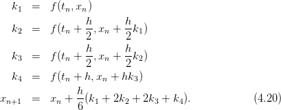
We note that the second term of the last equation takes an average of the four
derivatives with weights  ,
,  ,
,  and
and  respectively. A generic small
change in these values will increase the discretization error to worse than
 .
.
We remind to the reader the fact that by decreasing  the discretization
errors decrease, but that roundoff errors will start showing up for small enough
 . Therefore, a careful determination of
  that minimizes the total error
should be made by studying the dependence of the results as a function of
 .
.
4.3.1 A Program for the 4th Order Runge–Kutta
Consider the problem of the motion of a particle in one dimension. For
this, we have to integrate a system of two differential equations (4.5)
for two unknown functions of time  and
and  so
that
 | (4.21) |
In this case, equations (4.20) generalize to:
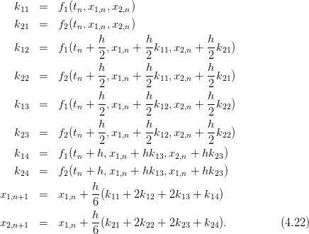
Programming this algorithm is quite simple. The main program is an interface
between the user and the driver routine of the integration. The user enters the
initial and final times  Ti and
  Tf and the number of discrete time
points Nt. The initial conditions are
  X10,
X10,  X20. The main data
structure consists of three global double arrays T[P], X1[P], X2[P] which store
the times
  and the corresponding values of the functions
 and
and  ,
,  . The main program calls the driver routine
RK(Ti,Tf,X10,X20,Nt) which “drives” the heart of the program, the function
RKSTEP(t,x1,x2,dt) which performs one integration step using equations (4.22)
. RKSTEP evolves the functions x1, x2 at time t by one step
  dt. The
function RK stores the calculated values in the arrays T, X1 and X2 at each
step. When RK returns the control to the main program, all the results
are stored in T, X1 and X2, which are subsequently printed in the file
rk.dat. The full program is listed below and can be found in the file
rk.cpp:
//========================================================
//Program to solve a 2 ODE system using Runge-Kutta Method
//User must supply derivatives
//dx1/dt=f1(t,x1,x2) dx2/dt=f2(t,x1,x2)
//as real functions
//Output is written in file rk.dat
//========================================================
#include <iostream>
#include <fstream>
#include <cstdlib>
#include <string>
#include <cmath>
using namespace std;
//--------------------------------------------------------
const int P = 110000;
double T[P], X1[P], X2[P];
//--------------------------------------------------------
double
f1(const double& t , const double& x1, const double& x2);
double
f2(const double& t , const double& x1, const double& x2);
void
RK(const double& Ti , const double& Tf, const double& X10,
const double& X20, const int & Nt);
void
RKSTEP(double& t, double& x1, double& x2,
const double& dt);
//--------------------------------------------------------
int main(){
double Ti,Tf,X10,X20;
int Nt;
int i;
string buf;
//Input:
cout << "Runge-Kutta Method for 2-ODEs Integration\n";
cout << "Enter Nt,Ti,TF,X10,X20:" << endl;
cin >> Nt >> Ti >> Tf >> X10 >> X20;getline(cin,buf);
cout << "Nt = " << Nt << endl;
cout << "Time: Initial Ti = " << Ti
<< " Final Tf = " << Tf << endl;
cout << " X1(Ti)= " << X10
<< " X2(Ti)= " << X20 << endl;
if(Nt >= P){cerr << "Error! Nt >= P\n";exit(1);}
//Calculate:
RK(Ti,Tf,X10,X20,Nt);
//Output:
ofstream myfile("rk.dat");
myfile.precision(17);
for(i=0;i<Nt;i++)
myfile << T [i] << " "
<< X1[i] << " "
<< X2[i] << ’\n’;
myfile.close();
}//main()
//========================================================
//The functions f1,f2(t,x1,x2) provided by the user
//========================================================
double
f1(const double& t, const double& x1, const double& x2){
return x2;
}
//--------------------------------------------------------
double
f2(const double& t, const double& x1, const double& x2){
return -10.0*x1; //harmonic oscillator
}
//========================================================
//RK(Ti,Tf,X10,X20,Nt) is the driver
//for the Runge-Kutta integration routine RKSTEP
//Input: Initial and final times Ti,Tf
// Initial values at t=Ti X10,X20
// Number of steps of integration: Nt-1
//Output: values in arrays T[Nt],X1[Nt],X2[Nt] where
//T[0] = Ti X1[0] = X10 X2[0] = X20
// X1[k-1] = X1(at t=T(k))
// X2[k-1] = X2(at t=T(k))
//T[Nt-1] = Tf
//========================================================
void
RK(const double& Ti , const double& Tf, const double& X10,
const double& X20, const int & Nt){
double dt;
double TS,X1S,X2S; //time and X1,X2 at given step
int i;
//Initialize variables:
dt = (Tf-Ti)/(Nt-1);
T [0] = Ti;
X1[0] = X10;
X2[0] = X20;
TS = Ti;
X1S = X10;
X2S = X20;
//Make RK steps: The arguments of RKSTEP are
//replaced with the new ones!
for(i=1;i<Nt;i++){
RKSTEP(TS,X1S,X2S,dt);
T [i] = TS;
X1[i] = X1S;
X2[i] = X2S;
}
}//RK()
//========================================================
//Function RKSTEP(t,x1,x2,dt)
//Runge-Kutta Integration routine of ODE
//dx1/dt=f1(t,x1,x2) dx2/dt=f2(t,x1,x2)
//User must supply derivative functions:
//real function f1(t,x1,x2)
//real function f2(t,x1,x2)
//Given initial point (t,x1,x2) the routine advances it
//by time dt.
//Input : Inital time t and function values x1,x2
//Output: Final time t+dt and function values x1,x2
//Careful!: values of t,x1,x2 are overwritten...
//========================================================
void
RKSTEP(double& t, double& x1, double& x2,
const double& dt){
double k11,k12,k13,k14,k21,k22,k23,k24;
double h,h2,h6;
h =dt; //h =dt, integration step
h2 =0.5*h; //h2=h/2
h6 =h/6.0; //h6=h/6
k11=f1(t,x1,x2);
k21=f2(t,x1,x2);
k12=f1(t+h2,x1+h2*k11,x2+h2*k21);
k22=f2(t+h2,x1+h2*k11,x2+h2*k21);
k13=f1(t+h2,x1+h2*k12,x2+h2*k22);
k23=f2(t+h2,x1+h2*k12,x2+h2*k22);
k14=f1(t+h ,x1+h *k13,x2+h *k23);
k24=f2(t+h ,x1+h *k13,x2+h *k23);
t =t+h;
x1 =x1+h6*(k11+2.0*(k12+k13)+k14);
x2 =x2+h6*(k21+2.0*(k22+k23)+k24);
}//RKSTEP()
4.4 Comparison of the Methods
In this section we will check our programs for correctness and accuracy w.r.t.
discretization and roundoff errors. The simplest test is to check the results against
a known analytic solution of a simple model. This will be done for the
simple harmonic oscillator. We will change the functions that compute the
acceleration of the particle to give  . We will take
  (
( ). Therefore the relevant part of the program in euler.cpp
becomes
double accel(const double& x){
return -10.0 * x;
}
and that of the program in rk.cpp becomes
double
f2(const double& t, const double& x1, const double& x2){
return -10.0*x1;
}
The programs are run for a given time interval  to
to  with the
initial conditions
  ,
,  . The time step
  is varied by
varying the number of steps Nt-1. The computed numerical solution is
compared to the well known solution for the simple harmonic oscillator
We study the deviation  and
and  as a
function of the time step
  . The results are shown in figures 4.11–4.14. We
note that for the Euler method and the Euler–Cromer method, the errors
are of order
  as expected. However, the latter has smaller errors
compared to the first one. For the Euler–Verlet method, the error turns out
to be of order
  whereas for the 4th order Runge–Kutta is of
order
 .
.
Another way for checking the numerical results is by looking at a conserved
quantity, like the energy, momentum or angular momentum, and study its
deviation from its original value. In our case we study the mechanical
energy
 | (4.24) |
which is computed at each step. The deviation  is shown in figures
4.15–4.18.
4.5 The Forced Damped Oscillator
In this section we will study a simple harmonic oscillator subject to a damping
force proportional to its velocity and an external periodic driving force,
which for simplicity will be taken to have a sinusoidal dependence in
time,
 | (4.25) |
where  and
and  is the angular frequency of the driving
force.
Consider initially the system without the influence of the driving
force, i.e. with  . The real solutions of the differential
equation
which are finite for
  are given by
 | (4.26) |
 | (4.27) |
In the last case, the solution oscillates with an amplitude decreasing exponentially
with time.
In the  case, the general solution is obtained from the sum of a special
solution
  and the solution of the homogeneous equation
  . A special
solution can be obtained from the ansatz
  ,
which when substituted in (4.25) and solved for
  and
and  we find
that
![a0 [(ω2 − ω2 )cosωt + γ ωsin ωt]
xs(t) = ------0--2----2-2----2-2-------,
(ω 0 − ω ) + ω γ](main_latex1716x.png) | (4.29) |
and
 | (4.30) |
The solution  decreases exponentially with time and eventually only
 remains. The only case where this is not true, is when we have
resonance without damping for
  ,
,  . In that case the solution
is
 | (4.31) |
The first two terms are the same as that of the simple harmonic oscillator. The
last one increases the amplitude linearly with time, which is a result of the influx
of energy from the external force to the oscillator.
Our program will be a simple modification of the program in rk.cpp. The
main routines RK(T0,TF,X10,X20,Nt) and RKSTEP(t,x1,x2,dt) remain as they
are. We only change the user interface. The basic parameters  ,
,  ,
,  ,
,  are entered interactively by the user from the standard input stdin. These
parameters should be accessible also by the function f2(t,x1,x2) and they are
declared within the global scope. Another point that needs our attention is
the function f2(t,x1,x2) which now takes the velocity
  x2 in its
arguments:
double
f2(const double& t, const double& x1, const double& x2){
double a;
a = a_0*cos(omega*t);
return -omega_02*x1-gam*x2+a;
}
The main program, found in the file dlo.cpp, is listed below. The functions RK,
RKSTEP are the same as in rk.cpp and should also be included in the same
file.
//========================================================
//Program to solve Damped Linear Oscillator
//using 4th order Runge-Kutta Method
//Output is written in file dlo.dat
//========================================================
#include <iostream>
#include <fstream>
#include <cstdlib>
#include <string>
#include <cmath>
using namespace std;
//--------------------------------------------------------
const int P = 110000;
double T[P], X1[P], X2[P];
double omega_0,omega,gam,a_0,omega_02,omega2;
//--------------------------------------------------------
double
f1(const double& t , const double& x1, const double& x2);
double
f2(const double& t , const double& x1, const double& x2);
void
RK(const double& Ti , const double& Tf, const double& X10,
const double& X20, const int & Nt);
void
RKSTEP(double& t, double& x1, double& x2,
const double& dt);
//--------------------------------------------------------
int main(){
double Ti,Tf,X10,X20;
double Energy;
int Nt;
int i;
string buf;
//Input:
cout << "Runge-Kutta Method for DLO Integration\n";
cout << "Enter omega_0, omega, gamma, a_0:\n";
cin >> omega_0>> omega>> gam>> a_0;getline(cin,buf);
omega_02 = omega_0*omega_0;
omega2 = omega *omega;
cout << "omega_0= " << omega_0
<< " omega= " << omega << endl;
cout << "gamma= " << gamma
<< " a_0= " << a_0 << endl;
cout << "Enter Nt,Ti,TF,X10,X20:" << endl;
cin >> Nt >> Ti >> Tf >> X10 >> X20;getline(cin,buf);
cout << "Nt = " << Nt << endl;
cout << "Time: Initial Ti = " << Ti
<< " Final Tf = " << Tf << endl;
cout << " X1(Ti)= " << X10
<< " X2(Ti)= " << X20 << endl;
if(Nt >= P){cerr << "Error! Nt >= P\n";exit(1);}
//Calculate:
RK(Ti,Tf,X10,X20,Nt);
//Output:
ofstream myfile("dlo.dat");
myfile.precision(17);
myfile << "# Damped Linear Oscillator - dlo\n";
myfile << "# omega_0= " << omega_0 << " omega= " << omega
<< " gamma= " << gam << " a_0= " << a_0 << endl;
for(i=0;i<Nt;i++){
Energy = 0.5*X2[i]*X2[i]+0.5*omega_02*X1[i]*X1[i];
myfile << T [i] << " "
<< X1[i] << " "
<< X2[i] << " "
<< Energy << ’\n’;
}
myfile.close();
}//main()
//========================================================
//The functions f1,f2(t,x1,x2) provided by the user
//========================================================
double
f1(const double& t, const double& x1, const double& x2){
return x2;
}
//--------------------------------------------------------
double
f2(const double& t, const double& x1, const double& x2){
double a;
a = a_0*cos(omega*t);
return -omega_02*x1-gam*x2+a;
}
The results are shown in figures 4.19–4.22. Figure 4.19 shows the transition
from a damped motion for  to an oscillating motion with damping
amplitude for
  . The exponential decrease of the amplitude is shown in
figure 4.21, whereas the dependence of the period
  from the damping coefficient
 is shown in figure 4.22. Motivated by equation (4.28) , written in the
form
 | (4.32) |
we construct the plot in figure 4.22. The right hand side of the equation is put on
the horizontal axis, whereas the left hand side on the vertical. Equation (4.32)
predicts that both quantities are equal and all measurements should lie on a
particular line, the diagonal  . The period
  can be estimated from the
time between two consecutive extrema of
  or two consecutive zeros of the
velocity
  (see figure 4.19).
Finally it is important to study the trajectory of the system in phase space. This can
be seen
in figure 4.20. A point in this space is a state of the system and a trajectory
describes the evolution of the system’s states in time. We see that all such
trajectories end up as  to the point
  , independently of the
initial conditions. Such a point is an example of a system’s attractor.
Next, we add the external force and study the response of the system to it.
The system exhibits a transient behavior that depends on the initial conditions.
For large enough times it approaches a steady state that does not depend
on (almost all of) the initial conditions. This can be seen in figure 4.23.
This is easily understood for our system by looking at equations (4.26) –
(4.28) . We see that the steady state  becomes dominant when
the exponentials have damped away.
  can be written in the form
These equations are verified in figure 4.24 where we study the dependence of the
amplitude  on the angular frequency of the driving force. Finally we study
the trajectory of the system in phase space. As we can see in figure 4.20, this time
the attractor is an ellipse, which is a one dimensional curve instead of a zero
dimensional point. For large enough times, all trajectories approach their
attractor asymptotically.
4.6 The Forced Damped Pendulum
In this section we will study a non-linear dynamical system which exhibits
interesting chaotic behavior. This is a simple model which, despite its
deterministic nature, the prediction of its future behavior becomes intractable
after a short period of time. Consider a simple pendulum in a constant
gravitational field whose motion is damped by a force proportional to its
velocity and it is under the influence of a vertical, harmonic external driving
force:
 | (4.34) |
In the equation above,  is the angle of the pendulum with the vertical axis,
  is the damping coefficient,
  is the pendulum’s natural angular
frequency,
  is the angular frequency of the driving force and
  is
the amplitude of the external angular acceleration caused by the driving
force.
In the absence of the driving force, the damping coefficient drives the system
to the point  , which is an attractor for the system. This continues
to happen for small enough
  , but for
  the behavior of the system
becomes more complicated.
The program that integrates the equations of motion of the system can be
obtained by making trivial changes to the program in the file dlo.cpp.
This changes are listed in detail below, but we note that X1  , X2
, X2
 , a_0
, a_0  . The final program can be found in the file fdp.cpp. It
is listed below, with the understanding that the commands in between
the dots are the same as in the programs found in the files dlo.cpp,
rk.cpp.
//========================================================
//Program to solve Forced Damped Pendulum
//using 4th order Runge-Kutta Method
//Output is written in file fdp.dat
//========================================================
................................
const int P = 1010000;
................................
Energy = 0.5*X2[i]*X2[i]+omega_02*(1.0-cos(X1[i]));
................................
double
f2(const double& t, const double& x1, const double& x2){
return -(omega_02+2.0*a_0*cos(omega*t))*sin(x1)-gam*x2;
}
................................
void
RKSTEP(double& t, double& x1, double& x2,
const double& dt){
................................
const double pi = 3.14159265358979324;
const double pi2= 6.28318530717958648;
x1 =x1+h6*(k11+2.0*(k12+k13)+k14);
x2 =x2+h6*(k21+2.0*(k22+k23)+k24);
if( x1 > pi ) x1 -= pi2;
if( x1 < -pi ) x1 += pi2;
}//RKSTEP()
The final lines in the program are added so that the angle is kept within the
interval ![[− π,π]](main_latex1783x.png) .
.
In order to study the system’s properties we will set  ,
,  , and
, and
 unless we explicitly state otherwise. The natural period of the pendulum
is
  whereas that of the driving force is
 . For
. For  , with
  , the
point
  is an attractor, which means that the pendulum eventually
stops at its stable equilibrium point. For
  the attractor is a
closed curve, which means that the pendulum at its steady state oscillates
indefinitely without circling through its unstable equilibrium point at
  .
The period of motion is found to be twice that of the driving force. For
 the attractor is an open curve, because at its steady state the
pendulum crosses the
  point. The period of the motion becomes
equal to that of the driving force. For
  we have period
doubling for critical values of
  , but the trajectory is still periodic. For
even larger values of
  the system enters into a chaotic regime where
the trajectories are non periodic. For
  we find the system in a
periodic steady state again, whereas for
  –
–  we have period
doubling. For
  we enter into a chaotic regime again etc. These
results can be seen in figures 4.27–4.29. The reader should construct the
bifurcation diagram of the system by solving problem 19 of this chapter.
We can also use the so called Poincaré diagrams in order to study the chaotic
behavior of a system. These are obtained by placing a point in phase
space when the time is an integer multiple of the period of the driving
force. Then, if for example the period of the motion is equal to that of
the period of the driving force, the Poincaré diagram consists of only
one point. If the period of the motion is an  –multiple of the period of
the driving force then the Poincaré diagram consists of only
  points.
Therefore, in the period doubling regime, the points of the Poincaré diagram
double at each period doubling point. In the chaotic regime, the Poincaré
diagram consists of an infinite number of points which belong to sets that
have interesting fractal structure. One way to construct the Poincaré
diagram numerically, is to process the data of the output file fdp.dat using
awk :
awk -v o=$omega -v nt=$Nt -v tf=$TF \
’BEGIN{T=6.283185307179/o;dt=tf/nt;} $1%T<dt{print $2,$3}’\
fdp.dat
where $omega, $Nt, $TF are the values of the angular frequency  ,
the number of points of time and the final time
  . We calculate
the period T and the time step dt in the program. Then we print
those lines of the file where the time is an integer multiple of the
period .
This is accomplished by the modulo operation $1 % T. The value of the
expression $1 % T < dt is true when the remainder of the division of the first
column ($1) of the file fdp.dat with the period T is smaller than dt. The results
in the chaotic regime are displayed in figure 4.30.
We close this section by discussing another concept that helps us in
the analysis of the dynamical properties of the pendulum. This is the
concept of the basin of attraction which is the set of initial conditions in
phase space that lead the system to a specific attractor. Take for example
the case for  in the regime where the pendulum at its steady
state has a circular trajectory with a positive or negative direction. By
taking a large sample of initial conditions and recording the direction of
the resulting motion after the transient behavior, we obtain figure 4.31.
4.7 Appendix: On the Euler–Verlet Method
Equations (4.11) can be obtained from the Taylor expansion
By adding and subtracting the above equations we obtain which give equations (4.11) From the first equation and equations (4.9) we obtain:
 | (4.37) |
When we perform a numerical integration, we are interested in the total error
accumulated after  integration steps. In this method, these errors must be
studied carefully:
Therefore the total error is  .
.
We also mention the Velocity Verlet method or the Leapfrog method. In this
case we use the velocity explicitly:
The last step uses the acceleration  which should depend only on the
position
  and not on the velocity.
The Verlet methods are popular in molecular dynamics simulations of many
body systems. One of their advantages is that the constraints of the system of
particles are easily encoded in the algorithm.
4.8 Appendix: 2nd order Runge–Kutta Method
In this appendix we will show how the choice of the intermediate point 2 in
equation (4.17) reduces the error by a power of  . This choice is special, since
by choosing another point (e.g.
  ) the result would have not been the
same. Indeed, from the relation
 | (4.40) |
By Taylor expanding around the point  we obtain
 | (4.41) |
Therefore
Note that for the vanishing of the  term it is necessary to place the
intermediate point at time
  .
.
This is not a unique choice. This can be most easily seen by a different
analysis of the Taylor expansion. Expanding around the point  we obtain
where we have set  ,
,  etc. We define and we will determine the conditions so that the terms
  of the last
equation in the error are identical with those of equation (4.43) . By expanding
 we obtain Substituting in (4.44) we obtain All we need is to choose The choice
  ,
,  ,
,  leads to equation (4.19) . Some other
choices in the bibliography are
  and
and  .
.
4.9 Problems
- Prove that the total error in the Euler–Cromer method is of order
 .
.
- Reproduce the results in figures 4.11–4.18
- Improve your programs so that there is no accumulation of roundoff
error in the calculation of time when h is very small for the
methods Euler, Euler-Cromer, Euler-Verlet and Runge-Kutta. Repeat
the analysis of the previous problem.
- Compare the results obtained from the Euler, Euler-Cromer, Euler-Verlet,
Runge-Kutta methods for the following systems where the analytic solution
is known:
- Particle falling in a constant gravitational field. Consider the case
 ,
,  ,
,  .
.
- Particle falling in a constant gravitational field moving in a fluid
from which exerts a force
 on the particle. Consider the
case
  ,
,  ,
, 
 . Calculate the
limiting velocity of the particle numerically and compare the value
obtained to the theoretical expectation.
- Repeat for the case of a force of resistance of magnitude
 .
.
- Consider the damped harmonic oscillator
 | (4.48) |
Take  ,
,  and calculate its mechanical energy as a
function of time. Is it monotonic? Why? (show that
  ).
Repeat for
  . When is the system oscillating and when it’s
not? Calculate numerically the critical value of
  for which the system
passes from a non oscillating to an oscillating regime. Compare your results
with the theoretical expectations.
- Reproduce the results of figures 4.19–4.22.
- Reproduce the results of figures 4.23–4.26. Calculate the phase
 numerically and compare with equation (4.33) .
- Consider a simple model for a swing. Take the damped harmonic oscillator
and a driving force which periodically exerts a momentary push with
angular frequency
 . Define “momentary” to be an impulse given by the
acceleration
  by an appropriately small time interval
  . The
acceleration is
  for all other times. Calculate the amplitude
  for
for
 and
and  .
.
- Consider a “half sine” driving force on a damped harmonic oscillator
 Study the transient behavior of the system for several initial conditions and
calculate its steady state motion for
  and
and  . Calculate
the amplitude
  .
.
- Consider the driving force on a damped oscillator given by
 Study the transient behavior of the system for several initial conditions and
calculate its steady state motion for
  and
and  . Calculate
the amplitude
  . Compare your results with those of the previous
problem and comment about.
- Write a program that simulates
 identical, independent harmonic
oscillators. Take
  and choose random initial conditions for each one
of them. Study their trajectories in phase space and check whether they
cross each other. Comment on your results.
- Place the
 harmonic oscillators of the previous problem in a
small square in phase space whose center is at the origin of the
axes. Consider the evolution of the system in time. Does the shape
of the rectangle change in time? Does the area change in time?
Explain...
- Repeat the previous problem when each oscillator is damped with
 .
Take
  .
.
- Consider the forced damped oscillator with
 ,
,  ,
,  .
Study the transient behavior of the system in the plots of
  ,
,  for
for
 .
.
- Consider the forced damped pendulum with
 ,
,  ,
,  and study the phase space trajectories for
  0.1, 0.19, 0.21, 0.25, 0.5,
0.71, 0.79, 0.85, 1.02, 1.031, 1.033, 1.05, 1.08, 1.1, 1.4, 1.8, 3.1, 3.5, 3.8, 4.2,
4.42, 4.44, 4.445, 4.447, 4.4488. Consider both the transient behavior and
the steady state motion.
- Reproduce the results in figures 4.30.
- Reproduce the results in figures 4.31.
- Consider the forced damped oscillator with
 After the transient behavior, the motion of the system for
  ,
,
 and
and  is periodic. Measure the period of the
motion with an accuracy of three significant digits and compare it
with the natural period of the pendulum and with the period of the
driving force. Take as initial conditions the following pairs:
 ,
,  ,
,  ,
,  ,
,  ,
,  ,
,
 ,
,  . Check if the period is independent of the initial
conditions.
- Consider the forced damped pendulum with
 Study the motion of the pendulum when the amplitude
  takes values in
the interval
 ![[0.2,5.0]](main_latex1937x.png) . Consider specific discrete values of
. Consider specific discrete values of  by splitting
the interval above in subintervals of width equal to
  .
For each value of
  , record in a file the value of
  , the angular
position and the angular velocity of the pendulum when
  with
with
 :
:
 The choice of
  is made so that the transient behavior will be
discarded and study only the steady state of the pendulum. You
may take
  ,
,  ,
,  ,
,  , and
split the intervals
 ![[tk,tk + π]](main_latex1950x.png) to 50 subintervals. Choose
to 50 subintervals. Choose  ,
,
 .
.
- Construct the bifurcation diagram by plotting the points
 .
.
- Repeat by plotting the points
 .
.
- Check whether your results depend on the choice of
 ,
,  .
Repeat your analysis for
  ,
,  .
.
- Study the onset of chaos: Take
![A ∈ [1.0000,1.0400]](main_latex1959x.png) with
with
 and
and ![A ∈ [4.4300,4.4500]](main_latex1961x.png) with
with  and
compute with the given accuracy the value
  where the system
enters into the chaotic behavior regime.
- The plot the points
 for
for 


 . Put 2000 points for each value of
  and
commend on the strength of the chaotic behavior of the pendulum.
Chapter 5
Planar Motion
In this chapter we will study the motion of a particle moving on the plane under
the influence of a dynamical field. Special emphasis will be given to the study of
the motion in a central field, like in the problem of planetary motion and
scattering. We also study the motion of two or more interacting particles moving
on the plane, which requires the solution of a larger number of dynamical
equations. These problems can be solved numerically by using Runge–Kutta
integration methods, therefore this chapter extends and applies the numerical
methods studied in the previous chapter.
5.1 Runge–Kutta for Planar Motion
In two dimensions, the initial value problem that we are interested in, is solving
the system of equations (4.6)
The 4th order Runge-Kutta method can be programmed by making small
modifications of the program in the file rk.cpp. In order to facilitate the study of
many different dynamical fields, for each field we put the code of the respective
acceleration in a different file. The code which is common for all the forces,
namely the user interface and the implementation of the Runge–Kutta method,
will be put in the file rk2.cpp. The program that computes the acceleration will
be put in a file named rk_XXX.cpp, where XXX is a string of characters that
identifies the force. For example, the file rk2_hoc.cpp contains the program
computing the acceleration of the simple harmonic oscillator, the file
rk2_g.cpp the acceleration of a constant gravitational field  etc.
etc.
Different force fields will require the use of one or more coupling constants
which need to be accessible to the code in the main program and some
subroutines. For this reason, we will provide two variables k1, k2 in the global
scope which will be accessed by the acceleration functions f3 and f4,
the function energy and the main program where the user will enter
their. The initial conditions are stored in the variables X10  , X20
, X20
 , V10
, V10  , V20
, V20  , and the values of the functions of
time will be stored in the arrays X1[P]
  , X2[P]
  , V1[P]
 , V2[P]
  . The integration is performed by a call to the
function RK(Ti,Tf,X10,X20,V10,V20,Nt) The results are written to the file
rk2.dat. Each line in this file contains the time, position, velocity and the
total mechanical energy, where the energy is calculated by the function
energy(t,x1,x2,v1,v2). The code for the function energy, which is different for
each force field, is written in the same file with the acceleration. The
code for the function RKSTEP(t,x1,x2,x3,x4,dt) should be extended in
order to integrate four instead of two functions. The full code is listed
below:
//========================================================
//Program to solve a 4 ODE system using Runge-Kutta Method
//User must supply derivatives
//dx1/dt=f1(t,x1,x2,x3,x4) dx2/dt=f2(t,x1,x2,x3,x4)
//dx3/dt=f3(t,x1,x2,x3,x4) dx4/dt=f4(t,x1,x2,x3,x4)
//as double functions
//Output is written in file rk2.dat
//========================================================
#include <iostream>
#include <fstream>
#include <cstdlib>
#include <string>
#include <cmath>
using namespace std;
//--------------------------------------------------------
const int P = 1010000;
double T[P], X1[P], X2[P], V1[P], V2[P];
double k1,k2;
//--------------------------------------------------------
double
f1(const double& t , const double& x1, const double& x2,
const double& v1 , const double& v2);
double
f2(const double& t , const double& x1, const double& x2,
const double& v1 , const double& v2);
double
f3(const double& t , const double& x1, const double& x2,
const double& v1 , const double& v2);
double
f4(const double& t , const double& x1, const double& x2,
const double& v1 , const double& v2);
double
energy
(const double& t , const double& x1, const double& x2,
const double& v1 , const double& v2);
void
RK(const double& Ti , const double& Tf ,
const double& X10, const double& X20,
const double& V10, const double& V20,
const int & Nt);
void
RKSTEP(double& t ,
double& x1, double& x2,
double& x3, double& x4,
const double& dt);
//--------------------------------------------------------
int main(){
string buf;
double Ti,Tf,X10,X20,V10,V20;
int Nt,i ;
double E0,EF,DE;
//Input:
cout << "Runge-Kutta Method for 4-ODEs Integration\n";
cout << "Enter coupling constants:\n";
cin >> k1 >> k2;getline(cin,buf);
cout << "k1= " << k1 << " k2= " << k2 << endl;
cout << "Enter Nt,Ti,Tf,X10,X20,V10,V20:\n";
cin >> Nt >> Ti >> Tf>> X10 >> X20 >> V10 >> V20;
getline(cin,buf);
cout << "Nt = " << Nt << endl;
cout << "Time: Initial Ti = " << Ti
<< " Final Tf= " << Tf << endl;
cout << " X1(Ti)= " << X10
<< " X2(Ti)=" << X20 << endl;
cout << " V1(Ti)= " << V10
<< " V2(Ti)=" << V20 << endl;
//Calculate:
RK(Ti,Tf,X10,X20,V10,V20,Nt);
ofstream myfile("rk2.dat");
myfile.precision(17);
for(i=0;i<Nt;i++)
myfile << T [i] << " "
<< X1[i] << " " << X2[i] << " "
<< V1[i] << " " << V2[i] << " "
<< energy(T[i],X1[i],X2[i],V1[i],V2[i])
<< endl;
myfile.close();
//Rutherford scattering angles:
cout.precision(17);
cout <<"v-angle: "<< atan2(V2[Nt-1],V1[Nt-1]) << endl;
cout <<"b-angle: "<< 2.0*atan(k1/(V10*V10*X20))<< endl;
E0=energy(Ti ,X10 ,X20 ,V10 ,V20 );
EF=energy(T[Nt-1],X1[Nt-1],X2[Nt-1],V1[Nt-1],V2[Nt-1]);
DE = abs(0.5*(EF-E0)/(EF+E0));
cout << "E0,EF, DE/E= " << E0
<< " " << EF
<< " " << DE << endl;
}//main()
//========================================================
//The velocity functions f1,f2(t,x1,x2,v1,v2)
//========================================================
double
f1(const double& t , const double& x1, const double& x2,
const double& v1, const double& v2){
return v1;
}
//--------------------------------------------------------
double
f2(const double& t , const double& x1, const double& x2,
const double& v1, const double& v2){
return v2;
}
//========================================================
//RK(Ti,Tf,X10,X20,V10,V20,Nt) is the driver
//for the Runge-Kutta integration routine RKSTEP
//Input: Initial and final times Ti,Tf
// Initial values at t=Ti X10,X20,V10,V20
// Number of steps of integration: Nt-1
// Size of arrays T,X1,X2,V1,V2
//Output: real arrays T[Nt],X1[Nt],X2[Nt],
// V1[Nt],V2[Nt] where
//T[0] = Ti X1[0] = X10 X2[0] = X20 V1[0] = V10 V2[0] = V20
// X1[k] = X1(at t=T[k]) X2[k] = X2(at t=T[k])
// V1[k] = V1(at t=T[k]) V2[k] = V2(at t=T[k])
//T[Nt-1]= Tf
//========================================================
void
RK(const double& Ti , const double& Tf ,
const double& X10, const double& X20,
const double& V10, const double& V20,
const int & Nt){
double dt;
double TS,X1S,X2S; //values of time and X1,X2 at given step
double V1S,V2S;
int i;
//Initialize:
dt = (Tf-Ti)/(Nt-1);
T [0] = Ti;
X1[0] = X10; X2[0] = X20;
V1[0] = V10; V2[0] = V20;
TS = Ti;
X1S = X10; X2S = X20;
V1S = V10; V2S = V20;
//Make RK steps: The arguments of RKSTEP are
//replaced with the new ones
for(i=1;i<Nt;i++){
RKSTEP(TS,X1S,X2S,V1S,V2S,dt);
T [i] = TS;
X1[i] = X1S; X2[i] = X2S;
V1[i] = V1S; V2[i] = V2S;
}
}//RK()
//========================================================
//Subroutine RKSTEP(t,x1,x2,dt)
//Runge-Kutta Integration routine of ODE
//dx1/dt=f1(t,x1,x2,x3,x4) dx2/dt=f2(t,x1,x2,x3,x4)
//dx3/dt=f3(t,x1,x2,x3,x4) dx4/dt=f4(t,x1,x2,x3,x4)
//User must supply derivative functions:
//real function f1(t,x1,x2,x3,x4)
//real function f2(t,x1,x2,x3,x4)
//real function f3(t,x1,x2,x3,x4)
//real function f4(t,x1,x2,x3,x4)
//Given initial point (t,x1,x2) the routine advances it
//by time dt.
//Input : Inital time t and function values x1,x2,x3,x4
//Output: Final time t+dt and function values x1,x2,x3,x4
//Careful: values of t,x1,x2,x3,x4 are overwritten...
//========================================================
void
RKSTEP(double& t ,
double& x1, double& x2,
double& x3, double& x4,
const double& dt){
double k11,k12,k13,k14,k21,k22,k23,k24;
double k31,k32,k33,k34,k41,k42,k43,k44;
double h,h2,h6;
h =dt; // h = dt, integration step
h2=0.5*h; // h2 = h/2
h6=h/6.0; // h6 = h/6
k11=f1(t,x1,x2,x3,x4);
k21=f2(t,x1,x2,x3,x4);
k31=f3(t,x1,x2,x3,x4);
k41=f4(t,x1,x2,x3,x4);
k12=f1(t+h2,x1+h2*k11,x2+h2*k21,x3+h2*k31,x4+h2*k41);
k22=f2(t+h2,x1+h2*k11,x2+h2*k21,x3+h2*k31,x4+h2*k41);
k32=f3(t+h2,x1+h2*k11,x2+h2*k21,x3+h2*k31,x4+h2*k41);
k42=f4(t+h2,x1+h2*k11,x2+h2*k21,x3+h2*k31,x4+h2*k41);
k13=f1(t+h2,x1+h2*k12,x2+h2*k22,x3+h2*k32,x4+h2*k42);
k23=f2(t+h2,x1+h2*k12,x2+h2*k22,x3+h2*k32,x4+h2*k42);
k33=f3(t+h2,x1+h2*k12,x2+h2*k22,x3+h2*k32,x4+h2*k42);
k43=f4(t+h2,x1+h2*k12,x2+h2*k22,x3+h2*k32,x4+h2*k42);
k14=f1(t+h ,x1+h *k13,x2+h *k23,x3+h *k33,x4+h *k43);
k24=f2(t+h ,x1+h *k13,x2+h *k23,x3+h *k33,x4+h *k43);
k34=f3(t+h ,x1+h *k13,x2+h *k23,x3+h *k33,x4+h *k43);
k44=f4(t+h ,x1+h *k13,x2+h *k23,x3+h *k33,x4+h *k43);
t =t+h;
x1=x1+h6*(k11+2.0*(k12+k13)+k14);
x2=x2+h6*(k21+2.0*(k22+k23)+k24);
x3=x3+h6*(k31+2.0*(k32+k33)+k34);
x4=x4+h6*(k41+2.0*(k42+k43)+k44);
}//RKSTEP()
5.2 Projectile Motion
Consider a particle in the constant gravitational field near the surface of the earth
which moves with constant acceleration  so that
 | (5.2) |
The particle moves on a parabolic trajectory that depends on the initial
conditions
where  is the direction of the initial velocity and
  is the
maximum height of the trajectory.
The acceleration 
 (
( f3 ,
f3 ,  f4) and the
mechanical energy is coded in the file rk2_g.cpp:
//========================================================
//The acceleration functions f3,f4(t,x1,x2,v1,v2) provided
//by the user
//========================================================
#include <iostream>
#include <fstream>
#include <cstdlib>
#include <string>
#include <cmath>
using namespace std;
extern double k1,k2;
//--------------------------------------------------------
//Free fall in constant gravitational field with
//g = -k2
double
f3(const double& t , const double& x1, const double& x2,
const double& v1, const double& v2){
return 0.0; // dx3/dt=dv1/dt=a1
}
//--------------------------------------------------------
double
f4(const double& t , const double& x1, const double& x2,
const double& v1, const double& v2){
return -k1; // dx4/dt=dv2/dt=a2
}
//--------------------------------------------------------
double
energy
(const double& t , const double& x1, const double& x2,
const double& v1, const double& v2){
return 0.5*(v1*v1+v2*v2) + k1*x2;
}
In order to calculate a projectile’s trajectory you may use the following
commands:
> g++ -O2 rk2.cpp rk2_g.cpp -o rk2
> ./rk2
Runge-Kutta Method for 4-ODEs Integration
Enter coupling constants:
10.0 0.0
k1= 10 k2= 0
Enter Nt,Ti,Tf,X10,X20,V10,V20:
20000 0.0 0.2 0.0 0.0 1.0 1.0
Nt = 20000
Time: Initial Ti = 0 Final Tf= 0.2
X1(Ti)= 0 X2(Ti)=0
V1(Ti)= 1 V2(Ti)=1
The analysis of the results contained in the file rk2.dat can be done using
gnuplot:
gnuplot> set terminal x11 1
gnuplot> plot "rk2.dat" using 1:2 with lines title "x(t)"
gnuplot> set terminal x11 2
gnuplot> plot "rk2.dat" using 1:3 with lines title "y(t)"
gnuplot> set terminal x11 3
gnuplot> plot "rk2.dat" using 1:4 with lines title "vx(t)"
gnuplot> set terminal x11 4
gnuplot> plot "rk2.dat" using 1:5 with lines title "vy(t)"
gnuplot> set terminal x11 5
gnuplot> plot "rk2.dat" using 1:($6-1.0) w lines t "E(t)-(0)"
gnuplot> set terminal x11 6
gnuplot> set size square
gnuplot> set title "Trajectory"
gnuplot> plot "rk2.dat" using 2:3 with lines notit
The results can be seen in figures 5.1 and 5.2. We note a small increase in
the mechanical energy which is due to the accumulation of numerical
errors.
We can animate the trajectory by writing a script of gnuplot commands in a
file rk2_animate.gpl
icount = icount+skip
plot "<cat -n rk2.dat" \
using 3:($1<= icount ? $4: 1/0) with lines notitle
# pause 1
if(icount < nlines ) reread
Before calling the script, the user must set the values of the variables
icount, skip and nlines. Each time gnuplot reads the script, it plots
icount number of lines from rk2.dat. Then the script is read again and a
new plot is made with skip lines more than the previous one, unless
icount < nlines. The plotted “file” "<cat -n rk2.dat" is the standard
output (stdout) of the command cat -n rk2.dat which prints to the
stdout the contents of the file rk2.dat line by line, together with the line
number. Therefore the plot command reads data which are the line number,
the time, the coordinate  , the coordinate
  etc. The keyword using
in
using 3:($1<= icount ? $4: 1/0)
instructs the plot command to use the 3rd column on the horizontal axis and if
the first column is less than icount ($1<= icount) put on the vertical axis the
value of the 4th column if the first column is less than icount. Otherwise ($1 >
icount) it prints an undefined number (1/0) which makes gnuplot print nothing
at all. You may also uncomment the command pause if you want to make
the animation slower. In order to run the script from gnuplot, issue the
commands
gnuplot> icount = 10
gnuplot> skip = 200
gnuplot> nlines = 20000
gnuplot> load "rk2_animate.gpl"
The scripts shown above can be found in the accompanying software. More
scripts can be found there that automate many of the boring procedures.
The usage of two of these is explained below. The first one is in the file
rk2_animate.csh:
> ./rk2_animate.csh -h
Usage: rk2_animate.csh -t [sleep time] -d [skip points] <file>
Default file is rk2.dat
Other options:
-x: set lower value in xrange
-X: set lower value in xrange
-y: set lower value in yrange
-Y: set lower value in yrange
-r: automatic determination of x-y range
> ./rk2_animate.csh -r -d 500 rk2.dat
The last line is a command that animates a trajectory read from the file
rk2.dat. Each animation frame contains 500 more points than the previous one.
The option -r calculates the plot range automatically. The option -h prints a
short help message.
A more useful script is in the file rk2.csh.
> ./rk2.csh -h
Usage: rk2.csh -f <force> k1 k2 x10 x20 v10 v20 STEPS t0 tf
Other Options:
-n Do not animate trajectory
Available forces (value of <force>):
1: ax=-k1 ay= -k2 y Harmonic oscillator
2: ax= 0 ay= -k1 Free fall
3: ax= -k2 vx ay= -k2 vy - k1 Free fall + \
air resistance ~ v
4: ax= -k2 |v| vx ay= -k2 |v|vy - k1 Free fall + \
air resistance ~ v^2
5: ax= k1*x1/r^3 ay= k1*x2/r^3 Coulomb Force
....
The option -h prints operating instructions. A menu of forces is available, and a
choice can be made using the option -f. The rest of the command line consists of
the parameters read by the program in rk2.cpp, i.e. the coupling constants k1,
k2, the initial conditions x10, x20, v10, v20 and the integration parameters
STEPS, t0 and tf. For example, the commands
[literate={-}{{\texttt{-}}}1]
> rk2.csh -f 2 -- 10.0 0.0 0.0 0.0 1.0 1.0 20000 0.0 0.2
> rk2.csh -f 1 -- 16.0 1.0 0.0 1.0 1.0 0.0 20000 0.0 6.29
> rk2.csh -f 5 -- 10.0 0.0 -10 0.2 10. 0.0 20000 0.0 3.00
compute the trajectory of a particle in the constant gravitational field discussed
above, the trajectory of an anisotropic harmonic oscillator (k1 =  ,
k2 =
  ) and the scattering of a particle in a Coulomb field –
try them! I hope that you will have enough curiosity to look “under the
hood” of the scripts and try to modify them or create new ones. Some
advise to the lazy guys: If you need to program your own force field follow
the recipe: Write the code of your acceleration field in a file named e.g.
rk2_myforce.cpp as we did with rk2_g.cpp. Edit the file rk2.csh and modify
the line
set forcecode = (hoc g vg v2g cb)
to
set forcecode = (hoc g vg v2g cb myforce)
(the variable $forcecode may have more entries than the ones shown
above). Count the order of the string myforce, which is 6 in our case. In
order to access this force field from the command line, use the option -f
6:
> rk2.csh -f 6 -- .......
Now, we will study the effect of the air resistance on the motion of the
projectile. For small velocities this is a force proportional to the velocity
 , therefore
By taking we obtain the motion of a particle with terminal velocity  (
( const.,
  ).
).
The acceleration caused by the air resistance is programmed in the file (k1
 , k2
, k2  ) rk2_vg.cpp:
//========================================================
//The acceleration functions f3,f4(t,x1,x2,v1,v2) provided
//by the user
//========================================================
//Free fall in constant gravitational filled with
//ax = -k2 vx ay = -k2 vy - k1
#include <iostream>
#include <fstream>
#include <cstdlib>
#include <string>
#include <cmath>
using namespace std;
extern double k1,k2;
//--------------------------------------------------------
double
f3(const double& t , const double& x1, const double& x2,
const double& v1, const double& v2){
return -k2*v1; // dx3/dt=dv1/dt=a1
}
//--------------------------------------------------------
double
f4(const double& t , const double& x1, const double& x2,
const double& v1, const double& v2){
return -k2*v2-k1; // dx4/dt=dv2/dt=a2
}
//--------------------------------------------------------
double
energy
(const double& t , const double& x1, const double& x2,
const double& v1, const double& v2){
return 0.5*(v1*v1+v2*v2) + k1*x2;
}
The results are shown in figure 5.3 where we see the effect of an increasing air
resistance on the particle trajectory. The effect of a resistance force of the form
 is shown in figure 5.4.
5.3 Planetary Motion
Consider the simple planetary model of a “sun” of mass  and a planet “earth”
at distance
  from the sun and mass
  such that
  . According to
Newton’s law of gravity, the earth’s acceleration is
 | (5.6) |
where  ,
,  ,
,  .
When the hypothesis
  is not valid, the two body problem is reduced to
that of the one body problem with the mass replaced by the reduced mass

 The force of gravity is a central force. This implies conservation of the angular
momentum
  with respect to the center of the force, which in turn
implies that the motion is confined on one plane. We choose the
  axis so
that
 | (5.7) |
The force of gravity is conservative and the mechanical energy
 | (5.8) |
is conserved. If we choose the origin of the coordinate axes to be the center of the
force, the equations of motion (5.6) become
where  . This is a system of two coupled differential equations for the
functions
  ,
,  . The trajectories are conic sections which are either an
ellipse (bound states - “planet”), a parabola (e.g. escape to infinity when the
particle starts moving with speed equal to the escape velocity) or a hyperbola
(e.g. scattering).
Kepler’s third law of planetary motion states that the orbital period  of a
planet satisfies the equation
 | (5.10) |
where  is the semi-major axis of the elliptical trajectory. The eccentricity is a
measure of the deviation of the trajectory from being circular
 | (5.11) |
where  is the semi-minor axis. The eccentricity is 0 for the circle and tends to 1
as the ellipse becomes more and more elongated. The foci
  and
and  are
located at a distance
  from the center of the ellipse. They have the property
that for every point on the ellipse
 | (5.12) |
The acceleration given to the particle by Newton’s force of gravity is
programmed in the file rk2_cb.cpp:
//========================================================
//The acceleration functions f3,f4(t,x1,x2,v1,v2) provided
//by the user
//========================================================
#include <iostream>
#include <fstream>
#include <cstdlib>
#include <string>
#include <cmath>
using namespace std;
extern double k1,k2;
//--------------------------------------------------------
//Motion in Coulombic potential:
//ax= k1*x1/r^3 ay= k1*x2/r^3
double
f3(const double& t , const double& x1, const double& x2,
const double& v1, const double& v2){
double r2,r3;
r2=x1*x1+x2*x2;
r3=r2*sqrt(r2);
if(r3>0.0)
return k1*x1/r3; // dx3/dt=dv1/dt=a1
else
return 0.0;
}
//--------------------------------------------------------
double
f4(const double& t , const double& x1, const double& x2,
const double& v1, const double& v2){
double r2,r3;
r2=x1*x1+x2*x2;
r3=r2*sqrt(r2);
if(r3>0.0)
return k1*x2/r3; // dx4/dt=dv4/dt=a4
else
return 0.0;
}
//--------------------------------------------------------
double
energy
(const double& t , const double& x1, const double& x2,
const double& v1, const double& v2){
double r;
r=sqrt(x1*x1+x2*x2);
if( r > 0.0)
return 0.5*(v1*v1+v2*v2) + k1/r;
else
return 0.0;
}
We set k1=  and take special care to avoid hitting the center of the
force, the singular point at
  . The same code can be used for the
electrostatic Coulomb field with k1=
  .
.
At first we study trajectories which are bounded. We set  ,
,
 ,
,  ,
,  and vary
  . We measure the period
  and
the length of the semi axes of the resulting ellipse. The results can be found in
table 5.1.
Some of the trajectories are shown in figure 5.5. There we can see the
dependence of the size of the ellipse on the period. Figure 5.6 confirms Kepler’s
third law of planetary motion given by equation (5.10) .
In order to confirm Kepler’s third law of planetary motion numerically, we
take the logarithm of both sides of equation (5.10)
 | (5.13) |
Therefore, the points  lie on a straight line. Using a linear least
squares fit we calculate the slope and the intercept which should be equal to
  and
and  respectively. This is left as an exercise.
In the case where the initial velocity of the particle becomes larger than the
escape velocity  , the particle escapes from the influence of the gravitational
field to infinity. The escape velocity corresponds to zero mechanical energy, which
gives
 | (5.14) |
When  ,
,  ,
,  , we obtain
  . The
numerical calculation of
  is left as an exercise.
5.4 Scattering
In this section we consider scattering of particles from a central
potential .
We assume particles that follow unbounded trajectories that start from infinity
and move almost free from the influence of the force field towards its center.
When they approach the region of interaction they get deflected and get
off to infinity in a new direction. We say that the particles have been
scattered and that the angle between their original and final direction is the
scattering angle  . Scattering problems are interesting because we can
infer to the properties of the scattering potential from the distribution of
the scattering angle. This approach is heavily used in today’s particle
accelerators for the study of fundamental interactions between elementary
particles.
First we will discuss scattering of small hard spheres of
radius  by other hard spheres or radius
  . The interaction
potential
is given by
 | (5.15) |
where  is the distance between the center of
  from the center of
  .
.
Assume that the particles in the beam do not interact with each other and
that there is only one collision per scattering. Let  be the intensity of the
beam
and
  its cross sectional area. Assume that the target has
  particles per unit
area. The cross sectional area of the interaction is
  where
where  and
and  are the radii of the scattered particles and targets respectively (see figure
(5.8) ): All the spheres of the beam which lie outside this area are not
scattered by the particular target. The total interaction cross section is
 | (5.16) |
where  is the total number of target spheres which lie within the beam. On
the average, the scattering rate is
 | (5.17) |
The above equation is the definition of the total scattering cross section  of the interaction. The differential cross section
  is defined by the
relation
 | (5.18) |
where  is the number of particles per unit time scattered within the solid
angle
  .
.
The total cross section is
 | (5.19) |
In the last relation we used the cylindrical symmetry of the interaction with
respect to the axis of the collision. Therefore
 | (5.20) |
This relation can be used in experiments for the measurement of the
differential cross section by measuring the rate of detection of particles within
the space contained in between two cones defined by the angles  and
and
 . This is the relation that we will use in the numerical calculation of
 .
.
Generally, in order to calculate the differential cross section we shoot a particle
at a target as shown in figure 5.9. The scattering angle  depends on the
impact parameter
  . The part of the beam crossing the ring of radius
 , thickness
  and area
  is scattered in angles between
  and
and  . Since there is only one particle at the target we have that
 . The number of particles per unit time crossing the ring is
  ,
therefore
 | (5.21) |
(the  sign is because as
  increases,
  decreases). From the potential we can
calculate
  and from
  we can calculate
  . Conversely, if we measure
 , we can calculate
  .
.
5.4.1 Rutherford Scattering
The scattering of a charged particle with charge  (“electron”) in a
Coulomb potential of a much heavier charge
  (“nucleus”) is called
Rutherford scattering. In this case, the interaction potential is given by
 | (5.22) |
which accelerates the particle with acceleration
 | (5.23) |
The energy of the particle is  and the magnitude of its angular
momentum is
  , where
  . The dependence of the impact parameter
on the scattering angle is [40]
 | (5.24) |
Using equation (5.21) we obtain
 | (5.25) |
Consider the scattering trajectories. The results for same charges are shown in
figure 5.10. A similar figure is obtained in the case of opposite charges. In the
latter case we have to take special care for small impact parameters  where the scattering angle is
  . A large number of integration steps
is needed in order to obtain the desired accuracy. A useful monitor of
the accuracy of the calculation is the measurement of the energy of the
particle which should be conserved. The results are shown in table 5.2.
Table 5.3: Rutherford scattering of opposite charges with  . The table is
similar to table 5.2. We observe the numerical difficulty for small impact parameters.
We will now describe a method for calculating the cross section by
using equation (5.20) . Alternatively we could have used equation (5.21)
and perform a numerical calculation of the derivatives. This is left as an
exercise for the reader. Our calculation is more like an experiment. We
place a “detector” that “detects” particles scattered within angles  and
and  . For this reason we split the interval
 ![[0,π ]](main_latex2326x.png) in
in  bins
so that
  . We perform “scattering experiments” by varying
![b ∈ [bm,bM ]](main_latex2329x.png) with step
with step  . Due to the symmetry of the problem we fix
  to be a constant, therefore a given
  corresponds to a cone with an
opening angle
  and an apex at the center of scattering. For given
  we
measure the scattering angle
  and record the number of particles per unit
time
  . The latter is proportional to the area of the ring of
radius
  . All we need now is the beam intensity
  which is the total
number of particles per unit time
  (note than in the ratio
 the proportionality constant and
  cancel) and the solid angle
 . Finally we can easily use equation (5.19) in order to calculate the
total cross section
  . The program that performs this calculation is in
the file scatter.cpp and it is a simple modification of the program in
rk2.cpp:
//========================================================
//Program that computes scattering cross-section of a central
//force on the plane. The user should first check that the
//parameters used, lead to a free state in the end.
// ** X20 is the impact parameter b **
//A 4 ODE system is solved using Runge-Kutta Method
//User must supply derivatives
//dx1/dt=f1(t,x1,x2,x3,x4) dx2/dt=f2(t,x1,x2,x3,x4)
//dx3/dt=f3(t,x1,x2,x3,x4) dx4/dt=f4(t,x1,x2,x3,x4)
//as real(8) functions
//Output is written in file scatter.dat
//========================================================
#include <iostream>
#include <fstream>
#include <cstdlib>
#include <string>
#include <cmath>
using namespace std;
//--------------------------------------------------------
const int P = 1010000;
double T[P], X1[P], X2[P], V1[P], V2[P];
double k1,k2;
//--------------------------------------------------------
double
f1(const double& t , const double& x1, const double& x2,
const double& v1 , const double& v2);
double
f2(const double& t , const double& x1, const double& x2,
const double& v1 , const double& v2);
double
f3(const double& t , const double& x1, const double& x2,
const double& v1 , const double& v2);
double
f4(const double& t , const double& x1, const double& x2,
const double& v1 , const double& v2);
double
energy
(const double& t , const double& x1, const double& x2,
const double& v1 , const double& v2);
void
RK(const double& Ti , const double& Tf ,
const double& X10, const double& X20,
const double& V10, const double& V20,
const int & Nt);
void
RKSTEP(double& t ,
double& x1, double& x2,
double& x3, double& x4,
const double& dt);
//--------------------------------------------------------
int main(){
string buf;
double Ti,Tf,X10,X20,V10,V20;
double X20F,dX20; //max impact parameter and step
int Nt,i ;
const int Nbins=20;
int index;
double angle,bins[Nbins],Npart;
const double PI =3.14159265358979324;
const double rad2deg=180.0/PI;
const double dangle =PI/Nbins;
double R,density,dOmega,sigma,sigmatot;
//Input:
cout << "Runge-Kutta Method for 4-ODEs Integration\n";
cout << "Enter coupling constants:\n";
cin >> k1 >> k2;getline(cin,buf);
cout << "k1= " << k1 << " k2= " << k2 << endl;
cout << "Enter Nt,Ti,Tf,X10,X20,V10,V20:\n";
cin >> Nt >> Ti >> Tf>> X10 >> X20 >> V10 >> V20;
getline(cin,buf);
cout << "Enter final impact parameter X20F and step dX20:\n";
cin >> X20F >> dX20;
cout << "Nt = " << Nt << endl;
cout << "Time: Initial Ti = " << Ti
<< " Final Tf= " << Tf << endl;
cout << " X1(Ti)= " << X10
<< " X2(Ti)=" << X20 << endl;
cout << " V1(Ti)= " << V10
<< " V2(Ti)=" << V20 << endl;
cout << "Impact par X20F =" << X20F
<< " dX20 =" << dX20 << endl;
ofstream myfile("scatter.dat");
myfile.precision(17);
for(i=0;i<Nbins;i++) bins[i] = 0.0;
//Calculate:
Npart = 0.0;
X20 = X20 + dX20/2.0; //starts in middle of first interval
while( X20 < X20F ){
RK(Ti,Tf,X10,X20,V10,V20,Nt);
//Take absolute value due to symmetry:
angle = abs(atan2(V2[Nt-1],V1[Nt-1]));
//Output: The final angle. Check if almost constant
myfile << "@ " << X20 << " " << angle
<< " " << abs(atan2(V2[Nt-51],V1[Nt-51]))
<< " " << k1/(V10*V10)/tan(angle/2.0) << endl;
//Update histogram:
index = int(angle/dangle);
//Number of incoming particles per unit time
//is proportional to radius of ring
//of radius X20, the impact parameter:
bins[index] += X20 ; // db is cancelled from density
Npart += X20 ; // <-- i.e. from here
X20 += dX20;
}//while( X20 < X20F )
//Print scattering cross section:
R = X20; //beam radius
density = Npart/(PI*R*R); //beam flux density J
sigmatot = 0.0; //total cross section
for(i=0;i<Nbins;i++){
angle = (i+0.5)*dangle;
dOmega = 2.0*PI*sin(angle)*dangle; //d(Solid Angle)
sigma = bins[i]/(density*dOmega);
if(sigma>0.0)
myfile << "ds= " << angle
<< " " << angle*rad2deg
<< " " << sigma << endl;
sigmatot += sigma*dOmega;
}//for(i=0;i<Nbins;i++)
myfile << "sigmatot= " << sigmatot << endl;
myfile.close();
}//main()
The results are recorded in the file scatter.dat. An example session that
reproduces figures 5.11 and 5.12 is
> g++ scatter.cpp rk2_cb.cpp -o scatter
> ./scatter
Runge-Kutta Method for 4-ODEs Integration
Enter coupling constants:
1.0 0.0
k1= 1 k2= 0
Enter Nt,Ti,Tf,X10,X20,V10,V20:
5000 0 30 -50 0.02 3 0
Enter final impact parameter X20F and step dX20:
1 0.0002
Nt = 5000
Time: Initial Ti = 0 Final Tf= 30
X1(Ti)= -50 X2(Ti)=0.02
V1(Ti)= 3 V2(Ti)=0
Impact par X20F =1 dX20 =0.0002
The results can be plotted with the gnuplot commands:
gnuplot> set log
gnuplot> plot [:1000] "<grep ds= scatter.dat" \
u ((sin($2/2))**(-4)):($4) notit,\
(1./(4.*3.**4))*x notit
gnuplot> unset log
gnuplot> set log y
gnuplot> plot [:] "<grep ds= scatter.dat" u 2:4 notit, \
(1./(4.*3.**4))*(sin(x/2))**(-4) notit
The results are in a very good agreement with the theoretical ones given by
(5.25) . The next step will be to study other central potentials whose solution is
not known analytically.
5.4.2 More Scattering Potentials
Consider scattering from a force field
 | (5.26) |
This is a very simple classical model of the scattering of a positron  by the
hydrogen atom. The positron has positive charge
  and the hydrogen atom
consists of a positively charged proton with charge
  in an electron
cloud of opposite charge
  . We set the scales so that
  and
and
 . We will perform a numerical calculation of
  ,
,  and
and
 .
.
The potential energy is given by
 | (5.27) |
where  for
for  . The program containing the calculation of the
acceleration caused by this force can be found in the file rk_hy.cpp:
//========================================================
//The acceleration functions f3,f4(t,x1,x2,v1,v2) provided
//by the user
//========================================================
#include <iostream>
#include <fstream>
#include <cstdlib>
#include <string>
#include <cmath>
using namespace std;
extern double k1,k2;
//--------------------------------------------------------
//Motion in hydrogen atom + positron:
//f(r) = 1/r^2-r/k1^3
//ax= f(r)*x1/r ay= f(r)*x2/r
double
f3(const double& t , const double& x1, const double& x2,
const double& v1, const double& v2){
double r2,r,fr;
r2=x1*x1+x2*x2;
r =sqrt(r2);
if(r <= k1 && r2 > 0.0)
fr = 1.0/r2-r/(k1*k1*k1);
else
fr = 0.0;
if(fr > 0.0 && r > 0.0)
return fr*x1/r; // dx3/dt=dv1/dt=a1
else
return 0.0;
}
//--------------------------------------------------------
double
f4(const double& t , const double& x1, const double& x2,
const double& v1, const double& v2){
double r2,r,fr;
r2=x1*x1+x2*x2;
r =sqrt(r2);
if(r <= k1 && r2 > 0.0)
fr = 1.0/r2-r/(k1*k1*k1);
else
fr = 0.0;
if(fr > 0.0 && r > 0.0)
return fr*x2/r; // dx4/dt=dv2/dt=a2
else
return 0.0;
}
//--------------------------------------------------------
double
energy
(const double& t , const double& x1, const double& x2,
const double& v1, const double& v2){
double r,Vr;
r=sqrt(x1*x1+x2*x2);
if(r <= k1 && r > 0.0)
Vr = 1/r + 0.5*r*r/(k1*k1*k1) - 1.5 / k1;
else
Vr = 0.0;
return 0.5*(v1*v1+v2*v2) + Vr;
}
The results are shown in figures 5.13–5.14. We find that  (see
problem 5.10).
Another interesting dynamical field is given by the Yukawa potential. This is a
phenomenological model of nuclear interactions:
 | (5.28) |
This field can also be used as a model of the effective interaction of electrons in
metals (Thomas–Fermi) or as the Debye potential in a classic plasma. The
resulting force is
 | (5.29) |
The program of the resulting acceleration can be found in the file rk2_yu.cpp.
The results are shown in figures 5.15–5.16.
5.5 More Particles
In this section we will generalize the discussion of the previous paragraphs in the
case of a dynamical system with more degrees of freedom. The number of
dynamical equations that need to be solved depends on the number of degrees of
freedom and we have to write a program that implements the 4th order
Runge–Kutta method for an arbitrary number of equations NEQ. We will explain
how to allocate memory dynamically, in which case the necessary memory storage
space, which depends on NEQ, is allocated at the time of running the program and
not at compilation time.
Until now, memory has been allocated statically. This means that arrays have
sizes which are known at compile time. For example, in the program rk2.cpp the
integer parameter P had a given value which determined the size of all arrays
using the declarations:
const int P = 1010000;
double T[P], X1[P], X2[P], V1[P], V2[P];
Changing P after compilation is impossible and if this becomes necessary we have
to edit the file, change the value of P and recompile. Dynamical memory allocation
allows us to read in Nt and NEQ at execution time and then ask from the operating
system to allocate the necessary memory. The needed memory can be asked
for at execution time by using the new operator. Here is an example:
double *T; //Declare 1-Dim arrays as pointers
double **X; //Declare 2-Dim arrays as pointers to pointers
int NEQ,Nt; //Variables of array sizes
//---------------------------------------------------------
finit(NEQ); //function that sets NEQ at run time
cin >> Nt; //read Nt at run time
//---------------------------------------------------------
//allocates 1-Dim array of Nt doubles
T = new double [Nt];
//allocates 1-Dim array of Nt pointers to doubles
X = new double*[Nt];
//for each i, allocate an array of NEQ doubles at X[i]:
for(int i=0;i<Nt;i++) X[i] = new double[NEQ];
.....
(compute with T[Nt], X[Nt][NEQ])
.....
//return allocated memory back to the system:
delete [] T; // deallocate an array
//for each i, deallocate the array of doubles X[i][NEQ]
for(int i=0;i<NEQ;i++) delete [] X[i];
//and then deallocate the array of pointers to doubles X[Nt]:
delete[] X ;
.....................
void finit(int& NEQ){//function that sets value of NEQ
NEQ = 4;
}
In this program, we should remember the fact that in C++, the name T of an
array T[Nt] is a pointer to T[0], which is denoted by &T[0]. This is the address
of the first element of the array in the memory. Therefore, if the array is
double T[Nt], then T is a pointer to a double: double *T. Then T+i
is a pointer to the address of the (i+1)-th element of the array T[i]
and
T+i = &T[i]
as well as
T[i] = *(T+i)
We can use pointers with the same notation as we do with arrays: If we declare a
pointer to a double *T1, and assign T1=T, then T1[0], T1[1], ... are the same
as T[0], T[1], .... For example, T1[0] = 2.0 assigns also T[0] and vice-versa.
Conversely, we can declare a pointer to a double *T, as we do in our program,
and make it point to a region in the memory where we have reserved space for Nt
doubles. This is what the operator new does. It asks for the memory for
Nt doubles and returns a pointer to it. Then we assign this pointer to
T:
double *T;
T = new double[Nt];
Then we can use T[0], T[1], ..., T[Nt-1] as we do with ordinary
arrays.
Two dimensional arrays are slightly trickier: For a two dimensional array,
double X[Nt][NEQ], X is a pointer to the value X[0][0], which is &X[0][0].
Then X[i] is a pointer to the one dimensional array X[i][NEQ], therefore X is a
pointer to a pointer of a double!
X[i][jeq] is: double
X[i] is: double *
X is: double **
Conversely, we can declare a double **X, and use the operator new to return a
pointer to an array of Nt pointers to doubles, and then for each element of the
array, use new to return a pointer to NEQ doubles:
double **X
X = new double*[Nt];
X[0] = new double[NEQ];
X[1] = new double[NEQ];
...
X[Nt-1] = new double[NEQ];
Then we can use the notation T[i][jeq], i= 0, 1, ..., Nt-1 and jeq= 0, 1,
..., NEQ-1, as we do with statically defined arrays.
The memory that we ask to be allocated dynamically is a finite resource that
can easily be exhausted (heard of memory leaks?). Therefore, we should be careful
to return unused memory to the system, so that it can be recycled. This should
happen especially within functions that we call many times, which allocate large
memory dynamically. The operator delete can be used to deallocate memory
that has been allocated with the operator new. For one dimensional arrays, this is
particularly simple:
double *T;
T = new double[Nt];
....
(use T[i])
...
delete [] T;
...
(cannot use T after delete)
For “two dimensional arrays” that have been allocated as we described above,
first we have to delete the arrays pointed by X[i] for i=0, ... , Nt-1, and then
the arrays of pointers pointed by X:
X = new double*[Nt ];
for(int i=0;i<Nt;i++) X[i] = new double[NEQ];
.... use X[i][jeq] ....
for(int i=0;i<NEQ;i++) delete [] X[i]; //delete all arrays X[i]
delete[] X ; //delete array of pointers
The main program will be written in the file rkA.cpp, whereas the
force-dependent part of the code will be written in files with names of the form
rkA_XXX.cpp. In the latter, the user must program a function f(t,X,dXdt) which
takes as input the time t and the values of the functions X[NEQ] and outputs the
values of their derivatives dXdt[NEQ] at time t. The function finit(NEQ) sets the
number of functions in f and it is called once during the initialization phase of the
program.
The program in the file rkA.cpp is listed below:
//========================================================
//Program to solve an ODE system using the
//4th order Runge-Kutta Method
//NEQ: Number of equations
//User supplies two functions:
//f(t,x,xdot): with double t,x[NEQ],xdot[NEQ] which
//given the time t and current values of functions x[NEQ]
//it returns the values of derivatives: xdot = dx/dt
//The values of two coupling constants k1,k2 may be used
//in f which are read in the main program
//finit(NEQ) : sets the value of NEQ
//
//User Interface:
//double k1,k2: coupling constants in global scope
//Nt,Ti,Tf: Nt-1 integration steps, initial/final time
//double X0[NEQ]: initial conditions
//Output:
//rkA.dat with Nt lines consisting of: T[Nt],X[Nt][NEQ]
//========================================================
#include <iostream>
#include <fstream>
#include <cstdlib>
#include <string>
#include <cmath>
using namespace std;
//--------------------------------------------------------
double *T; // T[Nt] stores the values of times
double **X; // X[Nt][NEQ] stores the values of functions
double k1,k2;
//--------------------------------------------------------
void RK(const double& Ti, const double& Tf, double* X0,
const int & Nt, const int & NEQ);
void RKSTEP( double& t , double* x ,
const double& dt, const int & NEQ);
//The following functions are defined in rkA_XX.cpp:
void finit( int & NEQ); //Sets number of equations
//Derivative and energy functions:
void f (const double& t, double* X,double* dXdt);
double energy(const double& t, double* X);
//--------------------------------------------------------
int main(){
string buf;
int NEQ,Nt;
double* X0;
double Ti,Tf;
//Get number of equations and allocate memory for X0:
finit(NEQ);
X0 = new double [NEQ];
//Input:
cout << "Runge-Kutta Method for ODE Integration.\n";
cout << "NEQ= " << NEQ << endl;
cout << "Enter coupling constants:\n";
cin >> k1 >> k2;getline(cin,buf);
cout << "k1= " << k1 << " k2= " << k2 << endl;
cout << "Enter Nt, Ti, Tf, X0:\n";
cin >> Nt>>Ti>>Tf;
for(int i=0;i<NEQ;i++) cin >> X0[i];getline(cin,buf);
cout << "Nt = " << Nt << endl;
cout << "Time: Initial Ti =" << Ti << " "
<< "Final Tf=" << Tf << endl;
cout << " X0 =";
for(int i=0;i<NEQ;i++) cout << X0[i] << " ";
cout << endl;
//Allocate memory for data arrays:
T = new double [Nt];
X = new double*[Nt];
for(int i=0;i<Nt;i++) X[i] = new double[NEQ];
//The Calculation:
RK(Ti,Tf,X0,Nt,NEQ);
//Output:
ofstream myfile("rkA.dat");
myfile.precision(16);
for(int i=0;i<Nt;i++){
myfile << T[i] << " ";
for(int jeq=0;jeq<NEQ;jeq++)
myfile << X[i][jeq] << " ";
myfile << energy(T[i],X[i]) << ’\n’;
}
myfile.close();
//------------------------------------------------------
//Cleaning up dynamic memory: delete[] each array
//created with the new operator (Not necessary in this
//program,it is done at the end of the program anyway)
delete[] X0;
delete[] T ;
for(int i=0;i<NEQ;i++) delete [] X[i];
delete[] X ;
}//main()
//========================================================
//Driver of the RKSTEP routine
//========================================================
void RK(const double& Ti, const double& Tf, double* X0,
const int & Nt, const int & NEQ){
double dt;
double TS;
double* XS;
XS = new double[NEQ];
//Initialize variables:
dt = (Tf-Ti)/(Nt-1);
T [0] = Ti;
for(int ieq=0;ieq<NEQ;ieq++) X[0][ieq]=X0[ieq];
TS = Ti;
for(int ieq=0;ieq<NEQ;ieq++) XS [ieq]=X0[ieq];
//Make RK steps: The arguments of RKSTEP are
//replaced with the new ones
for(int i=1;i<Nt;i++){
RKSTEP(TS,XS,dt,NEQ);
T[i] = TS;
for(int ieq=0;ieq<NEQ;ieq++) X[i][ieq] = XS[ieq];
}
// Clean up memory:
delete [] XS;
}//RK()
//========================================================
//Function RKSTEP(t,X,dt)
//Runge-Kutta Integration routine of ODE
//========================================================
void RKSTEP(double& t, double* x, const double& dt ,
const int & NEQ){
double tt;
double *k1, *k2, *k3, *k4, *xx;
double h,h2,h6;
k1 = new double[NEQ];
k2 = new double[NEQ];
k3 = new double[NEQ];
k4 = new double[NEQ];
xx = new double[NEQ];
h =dt; // h =dt, integration step
h2=0.5*h; // h2=h/2
h6=h/6.0; // h6=h/6
//1st step:
f(t ,x ,k1);
//2nd step:
for(int ieq=0;ieq<NEQ;ieq++)
xx[ieq] = x[ieq] + h2*k1[ieq];
tt =t+h2;
f(tt,xx,k2);
//3rd step:
for(int ieq=0;ieq<NEQ;ieq++)
xx[ieq] = x[ieq] + h2*k2[ieq];
tt =t+h2;
f(tt,xx,k3);
//4th step:
for(int ieq=0;ieq<NEQ;ieq++)
xx[ieq] = x[ieq] + h *k3[ieq];
tt=t+h ;
f(tt,xx,k4);
//Update:
t += h;
for(int ieq=0;ieq<NEQ;ieq++)
x[ieq] += h6*(k1[ieq]+2.0*(k2[ieq]+k3[ieq])+k4[ieq]);
//Clean up memory:
delete[] k1;
delete[] k2;
delete[] k3;
delete[] k4;
delete[] xx;
}//RKSTEP()
Consider three particles of equal mass exerting a force of gravitational attraction on
each other
like the ones shown in figure 5.17. The forces exerting on each other are given
by
 | (5.30) |
where  and the equations of motion become (
 )
)
where  . The total energy of the system is
 | (5.32) |
The relations shown above are programmed in the file rkA_3pcb.cpp listed
below:
#include <iostream>
#include <fstream>
#include <cstdlib>
#include <string>
#include <cmath>
using namespace std;
//--------------------------------------------------------
extern double k1,k2;
//--------------------------------------------------------
//Sets number of equations:
void finit(int& NEQ){
NEQ = 12;
}
//===============================
//Three particles of the same
//mass on the plane interacting
//via Coulombic force
//===============================
void f(const double& t, double* X,double* dXdt){
double x11,x12,x21,x22,x31,x32;
double v11,v12,v21,v22,v31,v32;
double r12,r13,r23;
//----------------
x11 = X[0];x21 = X[4];x31 = X[8];
x12 = X[1];x22 = X[5];x32 = X[9];
v11 = X[2];v21 = X[6];v31 = X[10];
v12 = X[3];v22 = X[7];v32 = X[11];
//----------------
r12 = pow((x11-x21)*(x11-x21)+(x12-x22)*(x12-x22),-3.0/2.0);
r13 = pow((x11-x31)*(x11-x31)+(x12-x32)*(x12-x32),-3.0/2.0);
r23 = pow((x21-x31)*(x21-x31)+(x22-x32)*(x22-x32),-3.0/2.0);
//----------------
dXdt[0] = v11;
dXdt[1] = v12;
dXdt[2] = k1*(x11-x21)*r12+k1*(x11-x31)*r13; // a11=dv11/dt
dXdt[3] = k1*(x12-x22)*r12+k1*(x12-x32)*r13; // a12=dv12/dt
//----------------
dXdt[4] = v21;
dXdt[5] = v22;
dXdt[6] = k1*(x21-x11)*r12+k1*(x21-x31)*r23; // a21=dv21/dt
dXdt[7] = k1*(x22-x12)*r12+k1*(x22-x32)*r23; // a22=dv22/dt
//----------------
dXdt[8] = v31;
dXdt[9] = v32;
dXdt[10] = k1*(x31-x11)*r13+k1*(x31-x21)*r23; // a31=dv31/dt
dXdt[11] = k1*(x32-x12)*r13+k1*(x32-x22)*r23; // a32=dv32/dt
}
//===============================
double energy(const double& t, double* X){
double x11,x12,x21,x22,x31,x32;
double v11,v12,v21,v22,v31,v32;
double r12,r13,r23;
double e;
//----------------
x11 = X[0];x21 = X[4];x31 = X[8];
x12 = X[1];x22 = X[5];x32 = X[9];
v11 = X[2];v21 = X[6];v31 = X[10];
v12 = X[3];v22 = X[7];v32 = X[11];
//----------------
r12 = pow((x11-x21)*(x11-x21)+(x12-x22)*(x12-x22),-0.5);
r13 = pow((x11-x31)*(x11-x31)+(x12-x32)*(x12-x32),-0.5);
r23 = pow((x21-x31)*(x21-x31)+(x22-x32)*(x22-x32),-0.5);
//----------------
e = 0.5*(v11*v11+v12*v12+v21*v21+v22*v22+v31*v31+v32*v32);
e += k1*(r12+r13+r23);
return e;
}
In order to run the program and see the results, look at the commands in the
shell script in the file rkA_3pcb.csh. In order to run the script use the
command
> rkA_3pcb.csh -0.5 4000 1.5 -1 0.1 1 0 1 -0.1 -1 0 0.05 1 0 -1
which will run the program setting  ,
,  ,
,  ,
,
 ,
,  ,
,  ,
,  , Nt
, Nt and
and  .
.
5.6 Problems
- Reproduce the results shown in figures 5.3 and 5.4. Compare your
results to the known analytic solution.
- Write a program for the force on a charged particle in a
constant magnetic field
 and compute its trajectory for
 . Set
. Set  and calculate the
resulting radius of the trajectory. Plot the relation between the radius
and
  . Compare your results to the known analytic solution. (assume
non relativistic motion)
- Consider the anisotropic
harmonic oscillator
 ,
,  . Construct the Lissajous
curves by setting
  ,
,  ,
,
 ,
,  . What happens when
  ?
?
- Reproduce the results displayed in table 5.1 and figures 5.5 and 5.6.
Plot
 vs
vs  and calculate the slope of the resulting straight
line by using the linear least squares method. Is it what you expect?
Calculate the intercept and compare your result with the expected one.
- Calculate the angular momentum with respect to the center of the force
at each integration step of the planetary motion and check whether it is
conserved. Show analytically that conservation of angular momentum
implies that the position vector sweeps areas at constant rate.
- Calculate the escape velocity of a planet
 for
for  ,
,
 ,
,  using the following steps: First show
that
  . Then set
  ,
,  . Vary
 and measure the resulting semi-major axis
  . Determine
the intercept of the resulting straight line in order to calculate
  .
.
- Repeat the previous problem for
 ,
,  ,
,  ,
,  ,
,  ,
,
 ,
,  ,
,  . From the
  plot confirm the relation
(5.14) .
- Check that for the bound trajectory of a planet with
 ,
,
 ,
,  ,
,  ,
,  you obtain that
 for each point
  of the trajectory. The point
  is the center of the force. After determining the semi-major axis
  numerically, the point
  will be taken symmetric to
  with respect
to the center of the ellipse.
- Consider the planetary motion studied in the previous problem. Apply
a momentary push in the tangential direction after the planet has
completed 1/4 of its elliptical orbit. How stable is the particle trajectory
(i.e. what is the dependence of the trajectory on the magnitude and
the duration of the push?)? Repeat the problem when the push is in
the vertical direction.
- Consider the scattering potential of the positron-hydrogen system
given by equation (5.26) . Plot the functions
 and
and  for
different values of
  . Calculate the total cross section
  numerically
and show that it is equal to
  .
.
- Consider the Morse potential of diatomic molecules:
 | (5.33) |
where  . Compute the solutions of the problem numerically in one
dimension and compare them to the known analytic solutions when
 :
:
 | (5.34) |
where the integration constant as a function of the initial position and
energy is given by
![[ αx0 ]
C = sin−1 ∘D--−-|E|e----- .
D(D − |E|)](main_latex2457x.png) | (5.35) |
We obtain a periodic motion with an energy dependent period
 . For
. For  we obtain
 | (5.36) |
whereas for 
 | (5.37) |
In these equations, the integration constant  is given by a different
relation and not by equation (5.35) . Compute the motion in phase space
 and study the transition from open to closed trajectories.
- Consider the effective potential term
 (
( ) in the
previous problem. Plot the function
  for
for  ,
,
 ,
,  ,
,  , and of course for
  . Determine the
equilibrium position and the ionization energy.
Calculate the solutions  ,
,  ,
,  ,
,  on the plane for
  ,
,
 , and
, and  numerically. In the
  case consider the scattering
problem and calculate the functions
  ,
,  and the total cross section
 .
.
- Consider the potential of the molecular model given by the force
 where
where  . Calculate the potential
 and plot the function
  . Determine the
equilibrium position and the ionization energy.
Consider the problem of scattering and calculate  ,
,  and
and  numerically. How much do your results depend on the minimum scattering
angle?
- Compute the trajectories of a particle under the influence of a force
 . Determine appropriate initial conditions that give a spiral
trajectory.
- Compute the total cross section
 for the Rutherford scattering both
analytically and numerically. What happens to your numerical results as you
vary the integration limits?
- Write a program that computes the trajectory of a particle that
moves on the plane in the static electric field of
 static point
charges.
- Solve the three body problem described in the text in the case of three
different electric charges by making the appropriate changes to the program
in the file rkA_3cb.cpp.
- Two charged particles of equal mass and charge are moving on the
 plane in a constant magnetic field
  . Solve the equations of motion
using a 4th order Runge–Kutta Method. Plot the resulting trajectories for
the initial conditions that you will choose.
- Three particles of equal mass
 are connected by identical springs. The
springs’ spring constant is equal to
  and their equilibrium length is equal
to
  . The particles move without friction on a horizontal plane. Solve the
equations of motion of the system numerically by using a 4th order
Runge–Kutta Method. Plot the resulting trajectories for the initial
conditions that you will choose. (Hint: Look in the files rkA_3hoc.cpp,
rkA_3hoc.csh.)
- Two identical particles are attached to thin weightless rods of length
 and they are connected by an ideal weightless spring with spring
constant
  and equilibrium length
  . The rods are hinged to the
ceiling at points whose distance is
  (see figure 5.18). Compute
the Lagrangian of the system and the equations of motion for the
degrees of freedom
  and
and  . Solve these equations numerically by
using a 4th order Runge–Kutta method. Plot the positions of the
particles in a Cartesian coordinate system and the resulting trajectory.
Study the normal modes for small angles
  and compute the
deviation of the solutions from the small oscillation approximation as
the angles become larger. (Hint: Look in the files rk_cpend.cpp,
rk_cpend.csh)
- Repeat the previous problem when the hinges of the rods slide without
friction on the
 axis.
axis.
- Repeat problem 5.20 by adding a third pendulum to the right at distance
 .
.
Chapter 6
Motion in Space
In this chapter we will study the motion of a
particle in space (three dimensions). We will also discuss the case of the
relativistic motion, which is important if one wants to consider the motion of
particles moving with speeds comparable to the speed of light. This will be an
opportunity to use an adaptive stepsize Runge-Kutta method for the numerical
solution of the equations of motion. We will use the open source code
rksuite available
at the Netlib
repository. Netlib is an open source, high quality repository for numerical analysis
software. The software it contains is used by many researchers in their high
performance computing programs and it is a good investment of time to learn how
to use it. Most of it is code written in Fortran and, in order to use it, you should
learn how to link a program written in C++ with functions written in a different
programming language.
The main technical skill that you will develop in this chapter is looking for
solutions to your numerical problems provided by software written by others. It is
important to be able to locate the optimal solution to your problem, find the
relevant functions, read the software’s documentation carefully and filter out
the necessary information in order to call and link the functions to your
program.
6.1 Adaptive Stepsize Control for RK Methods
The three dimensional equation of motion of a particle is an initial value problem
given by the equations (4.6)

For its numerical solution we will use an adaptive stepsize Runge–Kutta
algorithm for increased performance and accuracy. Adaptive stepsize is used in
cases where one needs to minimize computational effort for given accuracy goal.
The method frequently changes the time step during the integration process, so
that it is set to be large through smooth intervals and small when there are
abrupt changes in the values of the functions. This is achieved by exercising error
control, either by monitoring a conserved quantity or by computing the same
solution using two different methods. In our case, two Runge-Kutta methods are
used, one of order  and one of order
  , and the difference of the results
is used as an estimate of the truncation error. If the error needs to be
reduced, the step size is reduced and if it is satisfactorily small the step
size is increased. For the details we refer the reader to [33]. Our goal
is not to analyze and understand the details of the algorithm, but to
learn how to find and use appropriate and high quality code written by
others.
6.1.1 The rksuite Suite of RK Codes
The link http://www.netlib.org/ode/ reads
lib rksuite
alg Runge-Kutta
for initial value problem for first order ordinary differential
equations. A suite of codes for solving IVPs in ODEs. A
choice of RK methods, is available. Includes an error
assessment facility and a sophisticated stiffness checker.
Template programs and example results provided.
Supersedes RKF45, DDERKF, D02PAF.
ref RKSUITE, Softreport 92-S1, Dept of Math, SMU, Dallas, Texas
by R.W. Brankin (NAG), I. Gladwell and L.F. Shampine (SMU)
lang Fortran
prec double
There, we learn that the package provides code for Runge–Kutta methods, whose
source is open and written in the Fortran language. We also learn that the code is
written for double precision variables, which is suitable for our problem. Last, but
not least, we are also happy to learn that it is written by highly reputable people! We
download
the files rksuite.f, rksuite.doc, details.doc, templates, readme.
In order to link the subroutines provided by the suite to our program we need
to read the documentation carefully. In the general case, documentation is
available on the web (html, pdf, ...), bundled files with names like README and
INSTALL, in whole directories with names like doc/, online help in man and/or
info pages and, finally, in good old fashioned printed manuals. Good quality
software is also well documented inside the source code files, something that is
true for the software at hand.
In order to link the suite’s subroutines to our program we need the following
basic information:
- INPUT DATA: This is the necessary information that the program
needs in order to perform the calculation. In our case, the minimal
such information is the initial conditions, the integration time interval
and the number of integration steps. The user should also provide the
functions on the right hand side of (6.1) . It might also be necessary to
provide information about the desired accuracy goal, the scale of the
problem, the hardware etc.
- OUTPUT DATA: This is the information on how we obtain the
results of the calculation for further analysis. Information whether the
calculation was successful and error free could also be provided.
- WORKSPACE: This is information on how we provide the necessary
memory space used in the intermediate calculations. Such space needs
to be provided by the user in programming languages where dynamical
memory allocation is not possible, like in Fortran 77, and the size of
workspace depends on the parameters of the calling program.
It is easy to install the software. All the necessary code is in one file rksuite.f. The file
rksuite.doc
contains the documentation. There we read that we need to inform the program
about the hardware dependent accuracy of floating point numbers. We need to set
the values of three variables:
...
RKSUITE requires three environmental constants OUTCH, MCHEPS,
DWARF. When you use RKSUITE, you may need to know their
values. You can obtain them by calling the subroutine ENVIRN
in the suite:
CALL ENVIRN(OUTCH,MCHPES,DWARF)
returns values
OUTCH - INTEGER
Standard output channel on the machine being used.
MCHEPS - DOUBLE PRECISION
The unit of roundoff, that is, the largest
positive number such that 1.0D0 + MCHEPS = 1.0D0.
DWARF - DOUBLE PRECISION
The smallest positive number on the machine being
used.
...
************************** Installation Details ************
All machine-dependent aspects of the suite have been
isolated in the subroutine ENVIRN in the rksuite.f file.
...
The variables OUTCH, MCHEPS, DWARF are defined in the subroutine ENVIRN. They
are given generic default values but the programmer is free to change them by editing
ENVIRN. We should identify the routine in the file rksuite.f and read the comments
in it :
...
SUBROUTINE ENVIRN(OUTCH,MCHEPS,DWARF)
...
C The following six statements are to be Commented out
C after verification that the machine and installation
C dependent quantities are specified correctly.
...
WRITE(*,*) ’ Before using RKSUITE, you must verify that the ’
WRITE(*,*) ’ machine- and installation-dependent quantities ’
WRITE(*,*) ’ specified in the subroutine ENVIRN are correct, ’
WRITE(*,*) ’ and then Comment these WRITE statements and the ’
WRITE(*,*) ’ STOP statement out of ENVIRN. ’
STOP
...
C The following values are appropriate to IEEE
C arithmetic with the typical standard output channel.
C
OUTCH = 6
MCHEPS = 1.11D-16
DWARF = 2.23D-308
All we need to do is to comment out the WRITE and STOP commands since we will
keep the default values of the OUTCH, MCHEPS, DWARF variables:
...
C WRITE(*,*) ’ Before using RKSUITE, you must verify that the ’
C WRITE(*,*) ’ machine- and installation-dependent quantities ’
C WRITE(*,*) ’ specified in the subroutine ENVIRN are correct, ’
C WRITE(*,*) ’ and then Comment these WRITE statements and the ’
C WRITE(*,*) ’ STOP statement out of ENVIRN. ’
C STOP
...
In order to check whether the default values are satisfactory, we can
use the C++ template numeric_limits, which is part of the C++
Standard Library. In the file numericLimits.cpp, we write a small test
program :
#include <iostream>
#include <limits>
using namespace std;
int main(){
double MCHEPS,DWARF;
MCHEPS = numeric_limits<double>::epsilon();
DWARF = numeric_limits<double>::min ();
cout << "MCHEPS = " << MCHEPS/2.0 << endl;
cout << "DWARF = " << DWARF << endl;
}
We compile and run the above program as follows:
> g++ numericLimits.cpp -o n
> ./n
MCHEPS = 1.11022e-16
DWARF = 2.22507e-308
We conclude that our choices are satisfactory.
Next, we need to learn how to use the subroutines in the suite. By carefully
reading rksuite.doc we learn the following: The interface to the adaptive
stepsize Runge–Kutta algorithm is the routine UT (UT = “Usual Task”). The
routine can use a 2nd-3rd (RK23) order Runge-Kutta pair for error control
(METHOD=1), a 4th-5th (RK45) order pair (METHOD=2) or a 7th-8th (RK78) order
pair (METHOD=3). We will set METHOD=2 (RK45). The routine SETUP must be called
before UT for initialization. The user should provide a function F that calculates
the derivatives of the functions we integrate for, i.e. the right hand side of
6.1.
The fastest way to learn how to use the above routines is “by example”. The
suite include a templates package which can be unpacked by executing the
commands in the file templates using the sh shell:
> sh templates
tmpl1.out
tmpl1a.f
...
The file tmpl1a.f contains the solution of the simple harmonic oscillator and has
many explanatory comments in it. The code is in Fortran, but it is not so hard to
read. You may compile it and run it with the commands:
> cd rksuite/templates
> gfortran tmpl1a.f ../rksuite.f -o example1
> ./example1
We encourage the reader to study it carefully, run it and test its results.
6.1.2 Interfacing C++ Programs with Fortran
Next, we have to learn how to link the Fortran code in rksuite.f to a C++
program. There is a lot of relevant information that you can find with a simple
search in the web, we will concentrate on what is relevant to the program that we
need to write. The first thing that we need to learn is how to call a function
written in Fortran from a C++ program. A simple “Hello World” program can
teach us how to do it. Suppose that a Fortran function/subroutine HELLO() is
coded in a file helloF.f90:
SUBROUTINE HELLO()
PRINT *, ’Hello World!’
END SUBROUTINE HELLO
Then, we write in the file hello.cpp:
#include <iostream>
using namespace std;
extern "C" void hello_();
int main(){
hello_();
}
The first thing that we notice is that we call the function by lowering all letters
in its name: HELLO  hello. In Fortran, lowercase and uppercase letters are
equivalent, and the compiler creates names with lowercase letters only.
Next, we find that we need to append an underscore _ to the function’s
name :
hello
  hello_. The Fortran function needs to be declared in the “"C"
language linkage”:
extern "C" void hello_();
This is something one has to do both for functions written
in Fortran, as well as for functions written in plain old
C .
In order to compile and run the code we have to run the commands:
> gfortran -c helloF.f90
> g++ hello.cpp helloF.o -o hello -lgfortran
> ./hello
Hello World!
Compilation is done in two steps: We first need to compile the Fortran program using the
Fortran compiler
gfortran. The flag -c forces the compiler to perform compilation but not linking.
It produces an object file, whose extension is .o, helloF.o. These are files
which contain compiled code in non-readable text form, but they are not
autonomous executable programs. The functions that they contain, can be
linked to other compiled programs that call them. In the second step,
g++ is called to compile the C++ source code in hello.cpp and link
it to the functions in helloF.o. The flag -lgfortran is necessary in
order to link to the standard Fortran functions. If you use a different
compiler, you should read its manual in order to find the correct linking
options.
Another subtle point that needs to be considered is that, in Fortran, variables
are passed to functions by reference and not by value. Therefore, we have to pass
variables as pointers or as reference to variables. For example, the following Fortran
function
REAL (8) FUNCTION SQUAREMYDOUBLE(X)
REAL(8) x
X = 2.0*X
SQUAREMYDOUBLE = X*X
END FUNCTION SQUAREMYDOUBLE
must be declared and called as:
extern "C" double squaremydouble_(double& x);
...
double x,x2;
x2 = squaremydouble_(x);
For example, by modifying the hello.cpp program as
#include <iostream>
using namespace std;
extern "C" void hello_();
extern "C" double squaremydouble_(double& x);
int main(){
double x,x2;
hello_();
x = 2.0;
x2 = squaremydouble_(x);
cout << "x = " << 2.0 << endl;
cout << "2 x = " << x << endl;
cout << "(2 x)*(2 x) = " << x2 << endl;
}
we obtain the output:
> gfortran -c helloF.f90;
> g++ hello.cpp helloF.o -o hello -lgfortran
> ./hello
Hello World!
x = 2
2 x = 4
(2 x)*(2 x) = 16
Notice that the value of x is modified in the calling program.
The final issue that we will consider, it how to pass arrays to Fortran
functions. One dimensional arrays are quite easy to handle. In order to pass an
array double v[N] to a Fortran function, we only need to declare it and pass it as
one of its arguments. If the Fortran program is
real(8) function make_array1(v,N)
integer N
real(8) v(N)
... compute v(1) ... v(N) ...
end function make_array1
then the corresponding C++ program should be:
const int N=4;
extern "C" double make_array1_(double v[N], const int& N);
int main(){
double v[N], x;
...
x = make_array1_(v,N);
... use v[0] ... v[N-1] ...
}
The only point we need to stress is that the array real(8) v(N) is indexed from
1 to N in the Fortran program, whereas the array double v[N] is indexed
from 0 to N-1 in the C++ program. The correspondence of the values
stored in memory is v(1)  v[0], ... , v(i)
  v[i-1], ... v(N)
  v[N-1].
Two dimensional arrays need more attention. In C++, arrays are in row-major
mode, whereas in Fortran in column-major mode. The contents of a two
dimensional array are stored linearly in memory. In C++, the elements of an
array double A[N][M] are stored in the sequence A[0][0], A[0][1], A[0][2],
... , A[0][M-1], A[1][0], A[1][1], ... , A[1][M-1], ... A[N-1][M-1].
In Fortran, the elements of an array real(8) A(N,M) are stored in the sequence
A(1,1), A(2,1), A(3,1), ... , A(1,M), A(2,1), A(2,2), ... , A(2,M),
... , A(N,M). Therefore, when we pass an array from the C++ program to
a Fortran function, we have to keep in mind that the Fortran function
will use it with its indices transposed. For example, if the Fortran code
defines
A(i,j) = i + j/10.0
which results into A(i,j) = i.j in decimal
notation
(e.g. A(2,3)= 2.3), then the value of A[i][j] will be (j+1).(i+1) (e.g. A[2][3]
= 4.3, A[2][1] = 2.3)!
All of the above are summarized in the Fortran program in the file
CandFortranF.f90:
real(8) function make_array1(v,N)
implicit none
integer N,i
real(8) v(N)
do i=1,N
v(i) = i
end do
make_array1 = -11.0 ! a return value
end function make_array1
!----------------------------------------
real(8) function make_array2(A,N,M)
implicit none
integer N,M,i,j
real(8) A(M,N) ! Careful: N and M are interchanged!!
do i=1,M
do j=1,N
!A(i,j) = i.j, e.g. A(2,3)=2.3
A(i,j) = i + j/10.0
end do
end do
make_array2 = -22.0 ! a return value
end function make_array2
and the C++ program in the file CandFortranC.cpp:
#include <iostream>
#include <fstream>
#include <cstdlib>
#include <string>
#include <cmath>
using namespace std;
const int N=4, M=3;
extern "C" {
double make_array1_(double v[N] , const int& N);
double make_array2_(double A[N][M], const int& N,
const int& M);
}
int main(){
double A[N][M], v[N];
double x;
//Make a 1D array using a fortran function:
x = make_array1_(v,N);
cout << "1D array: Return value x= " << x << endl;
for(int i=0;i<N;i++)
cout << v[i] << " ";
cout << "\n-------------------------\n";
//Make an 2D array using a fortran function:
x = make_array2_(A,N,M);
cout << "2D array: Return value x= " << x << endl;
for(int i=0;i<N;i++){
for(int j=0;j<M;j++) //A is ... transposed!
//A[i][j] = (j+1).(i+1), e.g. A[1][2] = 3.1
cout << A[i][j] << " ";
cout << ’\n’;
}
}
Note that the array A[N][M] is defined as A(M,N) in the Fortran function, and
the roles of N and M are interchanged. You can run the code and see the output
with the commands:
> gfortran -c CandFortranF.f90
> g++ CandFortranC.cpp CandFortranF.o -o CandFortran -lgfortran
> ./CandFortran
1D array: Return value x= -11
1 2 3 4
-------------------------
2D array: Return value x= -22
1.1 2.1 3.1
1.2 2.2 3.2
1.3 2.3 3.3
1.4 2.4 3.4
Note that the values of the array A(M,N) are transposed when printed as rows in
the C++ program.
6.1.3 The rksuite Driver
After we become wise enough, we can write the driver for the integration routine
UT (called by ut_ from our C++ program), which can be found in the file
rk3.cpp:
//========================================================
//Program to solve a 6 ODE system using Runge-Kutta Method
//Output is written in file rk3.dat
//========================================================
// Compile with the commands:
// gfortran -c rksuite/rksuite.f;
// g++ rk3.cpp rk3_g.cpp rksuite.o -o rk3 -lgfortran
#include <iostream>
#include <fstream>
#include <cstdlib>
#include <string>
#include <cmath>
#include "rk3.h"
using namespace std;
//--------------------------------------------------------
double k1,k2,k3,k4;
double energy(const double& t, double* Y);
void f(double& t,double* Y, double* YP);
extern "C" {
void setup_(const int& NEQ,
double& TSTART,double* YSTART,double& TEND,
double& TOL ,double* THRES ,
const int& METHOD, const char& TASK,
bool & ERRASS,double& HSTART,double* WORK,
const int& LENWRK, bool& MESSAGE);
void ut_( void f(double& t,double* Y, double* YP),
double& TWANT, double& TGOT, double* YGOT,
double* YPGOT, double* YMAX, double* WORK,
int& UFLAG);
}
//--------------------------------------------------------
int main(){
string buf;
double T0,TF,X10,X20,X30,V10,V20,V30;
double t,dt,tstep;
int STEPS, i;
// rksuite variables:
double TOL,THRES[NEQ],WORK[LENWRK],HSTART;
double Y[NEQ],YMAX[NEQ],YP[NEQ],YSTART[NEQ];
bool ERRASS, MESSAGE;
int UFLAG;
const char TASK = ’U’;
//Input:
cout << "Runge-Kutta Method for 6-ODEs Integration\n";
cout << "Enter coupling constants k1,k2,k3,k4:\n";
cin >> k1 >> k2 >> k3 >> k4;getline(cin,buf);
cout << "Enter STEPS,T0,TF,X10,X20,X30,V10,V20,V30:\n";
cin >> STEPS >> T0 >> TF
>> X10 >> X20 >> X30
>> V10 >> V20 >> V30;getline(cin,buf);
cout << "No. Steps= " << STEPS << endl;
cout << "Time: Initial T0 =" << T0
<< " Final TF=" << TF << endl;
cout << " X1(T0)=" << X10
<< " X2(T0)=" << X20
<< " X3(T0)=" << X30 << endl;
cout << " V1(T0)=" << V10
<< " V2(T0)=" << V20
<< " V3(T0)=" << V30 << endl;
//Initial Conditions:
dt = (TF-T0)/STEPS;
YSTART[0] = X10;
YSTART[1] = X20;
YSTART[2] = X30;
YSTART[3] = V10;
YSTART[4] = V20;
YSTART[5] = V30;
//Set control parameters:
TOL = 5.0e-6;
for( i = 0; i < NEQ; i++)
THRES[i] = 1.0e-10;
MESSAGE = true;
ERRASS = false;
HSTART = 0.0;
//Initialization:
setup_(NEQ,T0,YSTART,TF,TOL,THRES,METHOD,TASK,
ERRASS,HSTART,WORK,LENWRK,MESSAGE);
ofstream myfile("rk3.dat");
myfile.precision(16);
myfile << T0<< " "
<< YSTART[0] << " " << YSTART[1] << " "
<< YSTART[2] << " " << YSTART[3] << " "
<< YSTART[4] << " " << YSTART[5] << " "
<< energy(T0,YSTART)<< ’\n’;
//The calculation:
for(i=1;i<=STEPS;i++){
t = T0 + i*dt;
ut_(f,t,tstep,Y,YP,YMAX,WORK,UFLAG);
if(UFLAG > 2) break; //error: break the loop and exit
myfile << tstep << " "
<< Y[0] << " " << Y[1] << " "
<< Y[2] << " " << Y[3] << " "
<< Y[4] << " " << Y[5] << " "
<< energy(T0,Y) << ’\n’;
}
myfile.close();
}// main()
All common parameters and variables are declared in an include file rk3.h.
This is done so that they are accessible by the function f which calculates the
derivatives:
const int NEQ = 6;
const int LENWRK = 32*NEQ;
const int METHOD = 2;
extern double k1,k2,k3,k4;
The number of differential equations is set equal to NEQ=6. The integration
method is set by the choice METHOD=2. The variable LENWRK sets the size of the
workspace needed by the suite for the intermediate calculations.
The declaration of functions needs some care. The functions energy() and f()
are defined in the C++ program and are declared in the global scope
(the function f() will also be passed on to the Fortran function UT). The
functions setup_() and ut_() are defined in the Fortran program in the file
rksuite.f as SETUP() and UT(). Therefore, they are declared within
the extern "C" language linkage, defined using lowercase letters and
an underscore is appended to their names. All arguments are passed by
reference. Scalar doubles are passed as references to double&, the double
precision arrays are declared to be pointers double *, the Fortran logical
variables are declared to be references to bool&, and the Fortran character*
variables
as simple references to char&.
The main program starts with the user interface. The initial state of the
particle is stored in the array YSTART in the positions  . The first three
positions are the coordinates of the initial position and the last three
the components of the initial velocity. Then, we set some variables that
determine the behavior of the integration program (see the file rksuite.doc
for details) and call the subroutine SETUP. The main integration loop
is:
for(i=1;i<=STEPS;i++){
t = T0 + i*dt;
ut_(f,t,tstep,Y,YP,YMAX,WORK,UFLAG);
if(UFLAG > 2) break; //error: break the loop and exit
myfile << ... << energy(T0,Y) << ’\n’;
}
The function f calculates the derivatives and it will be programmed by us later.
The variable t stores the desired moment of time at which we want to calculate
the functions. Because of the adaptive stepsize, it can be different than the one
returned by the Fortran subroutine UT. The actual value of time that the next step
lands
on is tstep. The array Y stores the values of the functions. We choose the data
structure to be such that  = Y[0],
  = Y[1],
  = Y[2] and
  = Y[3],
  =
Y[4],
  = Y([5] (the same sequence as in the array YSTART). The function
energy(t,Y) returns the value of the mechanical energy of the particle and its
code will be written in the same file as that of f. Finally, the variable UFLAG
indicates the error status of the calculation by UT and if UFLAG
 we end the
calculation.
Our test code will be on the study of the motion of a projectile in a
constant gravitational field, subject also to the influence of a dissipative force
 . The program is in the file rk3_g.cpp. We choose the parameters k1
and k2 so that
  -k1
-k1  and
and  k2.
k2.
#include <iostream>
#include <fstream>
#include <cstdlib>
#include <string>
#include <cmath>
#include "rk3.h"
using namespace std;
void f(double& t,double* Y, double* YP){
double x1,x2,x3,v1,v2,v3;
x1 = Y[0]; v1 = Y[3];
x2 = Y[1]; v2 = Y[4];
x3 = Y[2]; v3 = Y[5];
//Velocities: dx_i/dt = v_i
YP[0] = v1;
YP[1] = v2;
YP[2] = v3;
//Acceleration: dv_i/dt = a_i
YP[3] = -k2*v1;
YP[4] = -k2*v2;
YP[5] = -k2*v3-k1;
}
//---------------------------------
double energy(const double& t, double* Y){
double e;
double x1,x2,x3,v1,v2,v3;
x1 = Y[0]; v1 = Y[3];
x2 = Y[1]; v2 = Y[4];
x3 = Y[2]; v3 = Y[5];
//Kinetic Energy:
e = 0.5*(v1*v1+v2*v2+v3*v3);
//Potential Energy:
e += k1*x3;
return e;
}
For convenience we “translated” the values in the array Y[NEQ] into user-friendly
variable names. If the file rksuite.f is in the directory rksuite/, then the
compilation, running and visualization of the results can be done with the
commands:
> gfortran -c rksuite/rksuite.f
> g++ rk3.cpp rk3_g.cpp rksuite.o -o rk3 -lgfortran
> ./rk3
Runge-Kutta Method for 6-ODEs Integration
Enter coupling constants k1,k2,k3,k4:
10 0 0 0
Enter STEPS,T0,TF,X10,X20,X30,V10,V20,V30:
10000 0 3 0 0 0 1 1 1
No. Steps= 10000
Time: Initial T0 =0 Final TF=3
X1(T0)=0 X2(T0)=0 X3(T0)=0
V1(T0)=1 V2(T0)=1 V3(T0)=1
> gnuplot
gnuplot> plot "rk3.dat" using 1:2 with lines title "x1(t)"
gnuplot> plot "rk3.dat" using 1:3 with lines title "x2(t)"
gnuplot> plot "rk3.dat" using 1:4 with lines title "x3(t)"
gnuplot> plot "rk3.dat" using 1:5 with lines title "v1(t)"
gnuplot> plot "rk3.dat" using 1:6 with lines title "v2(t)"
gnuplot> plot "rk3.dat" using 1:7 with lines title "v3(t)"
gnuplot> plot "rk3.dat" using 1:8 with lines title "E(t)"
gnuplot> set title "trajectory"
gnuplot> splot "rk3.dat" using 2:3:4 with lines notitle
All the above commands can be executed together using the shell script in the file
rk3.csh. The script uses the animation script rk3_animate.csh. The following
command executes all the commands shown above:
./rk3.csh -f 1 -- 10 0. 0 0 0 0 0 1 1 1 10000 0 3
6.2 Motion of a Particle in an EM Field
In this section we study the non-relativistic motion of a charged particle in an
electromagnetic (EM) field. The particle is under the influence of the Lorentz
force:
 | (6.2) |
Consider the constant EM field of the form  ,
,  .
The components of the acceleration of the particle are:
This field is programmed in the file rk3_B.cpp. We set k1  , k2
, k2
 , k3
, k3  and k4
  :
:
//========================================================
// Particle in constant magnetic and electric field
// q B/m = k1 z q E/m = k2 x + k3 y + k4 z
//========================================================
#include "sr.h"
void f(double& t,double* Y, double* YP){
double x1,x2,x3,v1,v2,v3,p1,p2,p3;
x1 = Y[0]; p1 = Y[3];
x2 = Y[1]; p2 = Y[4];
x3 = Y[2]; p3 = Y[5];
velocity(p1,p2,p3,v1,v2,v3);
//now we can use all x1,x2,x3,p1,p2,p3,v1,v2,v3
YP[0] = v1;
YP[1] = v2;
YP[2] = v3;
//Acceleration:
YP[3] = k2 + k1 * v2;
YP[4] = k3 - k1 * v1;
YP[5] = k4;
}
//---------------------------------
double energy(const double& t, double* Y){
double e;
double x1,x2,x3,v1,v2,v3,p1,p2,p3,psq;
x1 = Y[0]; p1 = Y[3];
x2 = Y[1]; p2 = Y[4];
x3 = Y[2]; p3 = Y[5];
psq= p1*p1+p2*p2+p3*p3;
//Kinetic Energy:
e = sqrt(1.0+psq)-1.0;
//Potential Energy/m_0
e += - k2*x1 - k3*x2 - k4*x3;
return e;
}
We can also study space-dependent fields in the same way. The fields must
satisfy Maxwell’s equations. We can study the confinement of a particle in
a region of space by a magnetic field by taking  with
with
 ,
,  and
and  ,
,  .
Note that
  . You may also want to calculate the current density from
the equation
  .
.
The results are shown in figures 6.1–6.4.
6.3 Relativistic Motion
Consider a particle of non zero rest mass moving with speed
comparable to the speed of light. In this case, it is necessary to
study its motion using the equations of motion given by special
relativity .
In the equations below we set  . The particle’s rest mass is
  , its
mass is
  (where
  ), its momentum is
  and its
energy is
  . Then the equations of motion in a dynamic field
 are given by:
 | (6.4) |
In order to write a system of first order equations, we use the relations
 | (6.5) |
Using  we obtain
which is a system of first order differential equations for the functions 


 . Given the initial conditions


 their solution is
unique and it can be computed numerically using the 4th-5th order Runge–Kutta
method according to the discussion of the previous section. By using the relations
we can use the initial conditions
  ,
,  ,
,  ,
,  ,
,  ,
,  instead. Similarly, from the solutions
  ,
,  ,
,  ,
,  ,
,
 ,
,  we can calculate
  ,
,  ,
,  ,
,  ,
,  ,
,
 . We always have to check that
 | (6.8) |
Since half of the functions that we integrate for are the momentum instead of
the velocity components, we need to make some modifications to the
program in the file rk3.cpp. The main program can be found in the file
sr.cpp:
//========================================================
//Program to solve a 6 ODE system using Runge-Kutta Method
//Output is written in file sr.dat
//========================================================
// Compile with the commands:
// gfortran -c rksuite/rksuite.f
// g++ sr.cpp sr_B.cpp rksuite.o -o rk3 -lgfortran
//--------------------------------------------------------
#include "sr.h"
double k1,k2,k3,k4;
extern "C" {
void setup_(const int& NEQ,
double& TSTART,double* YSTART,double& TEND,
double& TOL ,double* THRES ,
const int& METHOD, const char& TASK,
bool & ERRASS,double& HSTART,double* WORK,
const int& LENWRK, bool& MESSAGE);
void ut_( void f(double& t,double* Y, double* YP),
double& TWANT, double& TGOT, double* YGOT,
double* YPGOT, double* YMAX, double* WORK,
int& UFLAG);
}
//--------------------------------------------------------
int main(){
string buf;
double T0,TF,X10,X20,X30,V10,V20,V30;
double P10,P20,P30;
double P1,P2,P3,V1,V2,V3;
double t,dt,tstep;
int STEPS, i;
// rksuite variables:
double TOL,THRES[NEQ],WORK[LENWRK],HSTART;
double Y[NEQ],YMAX[NEQ],YP[NEQ],YSTART[NEQ];
bool ERRASS, MESSAGE;
int UFLAG;
const char TASK = ’U’;
//Input:
cout << "Runge-Kutta Method for 6-ODEs Integration\n";
cout << "Special Relativistic Particle:\n";
cout << "Enter coupling constants k1,k2,k3,k4:\n";
cin >> k1 >> k2 >> k3 >> k4;getline(cin,buf);
cout << "Enter STEPS,T0,TF,X10,X20,X30,V10,V20,V30:\n";
cin >> STEPS >> T0 >> TF
>> X10 >> X20 >> X30
>> V10 >> V20 >> V30;getline(cin,buf);
momentum(V10,V20,V30,P10,P20,P30);
cout << "No. Steps= " << STEPS << endl;
cout << "Time: Initial T0 =" << T0
<< " Final TF=" << TF << endl;
cout << " X1(T0)=" << X10
<< " X2(T0)=" << X20
<< " X3(T0)=" << X30 << endl;
cout << " V1(T0)=" << V10
<< " V2(T0)=" << V20
<< " V3(T0)=" << V30 << endl;
cout << " P1(T0)=" << P10
<< " P2(T0)=" << P20
<< " P3(T0)=" << P30 << endl;
//Initial Conditions:
dt = (TF-T0)/STEPS;
YSTART[0] = X10;
YSTART[1] = X20;
YSTART[2] = X30;
YSTART[3] = P10;
YSTART[4] = P20;
YSTART[5] = P30;
//Set control parameters:
TOL = 5.0e-6;
for( i = 0; i < NEQ; i++)
THRES[i] = 1.0e-10;
MESSAGE = true;
ERRASS = false;
HSTART = 0.0;
//Initialization:
setup_(NEQ,T0,YSTART,TF,TOL,THRES,METHOD,TASK,
ERRASS,HSTART,WORK,LENWRK,MESSAGE);
ofstream myfile("sr.dat");
myfile.precision(16);
myfile << T0 << " "
<< YSTART[0] << " " << YSTART[1] << " "
<< YSTART[2] << " "
<< V1 << " " << V2 << " "
<< V3 << " "
<< energy(T0,YSTART) << " "
<< YSTART[3] << " " << YSTART[4] << " "
<< YSTART[5] << ’\n’;
//The calculation:
for(i=1;i<=STEPS;i++){
t = T0 + i*dt;
ut_(f,t,tstep,Y,YP,YMAX,WORK,UFLAG);
if(UFLAG > 2) break; //error: break the loop and exit
velocity(Y[3],Y[4],Y[5],V1,V2,V3);
myfile << tstep << " "
<< Y[0] << " " << Y[1] << " "
<< Y[2] << " "
<< V1 << " " << V2 << " "
<< V3 << " "
<< energy(T0,Y) << " "
<< Y[3] << " " << Y[4] << " "
<< Y[5] << " " << ’\n’;
}
myfile.close();
}// main()
//========================================================
//momentum -> velocity transformation
//========================================================
void velocity(const double& p1,const double& p2,
const double& p3,
double& v1, double& v2,
double& v3){
double psq;
psq = p1*p1+p2*p2+p3*p3;
v1 = p1/sqrt(1.0+psq);
v2 = p2/sqrt(1.0+psq);
v3 = p3/sqrt(1.0+psq);
}
//========================================================
//velocity -> momentum transformation
//========================================================
void momentum(const double& v1,const double& v2,
const double& v3,
double& p1, double& p2,
double& p3){
double vsq;
vsq = v1*v1+v2*v2+v3*v3;
if(vsq >= 1.0){cerr << "momentum: vsq>=1\n";exit(1);}
p1 = v1/sqrt(1.0-vsq);
p2 = v2/sqrt(1.0-vsq);
p3 = v3/sqrt(1.0-vsq);
}
The functions momentum and velocity compute the transformations (6.7) . In
the function momentum we check whether the condition (6.8) is satisfied. These
functions are also used in the function F that computes the derivatives of the
functions.
Common declarations are now in an include file sr.h:
#include <iostream>
#include <fstream>
#include <cstdlib>
#include <string>
#include <cmath>
using namespace std;
//---------------------------------------------
const int NEQ = 6;
const int LENWRK = 32*NEQ;
const int METHOD = 2;
extern double k1,k2,k3,k4;
//---------------------------------------------
double energy(const double& t, double* Y);
void f(double& t, double* Y, double* YP);
void velocity(const double& p1,const double& p2,
const double& p3,
double& v1, double& v2,
double& v3);
void momentum(const double& v1,const double& v2,
const double& v3,
double& p1, double& p2,
double& p3);
The test drive of the above program is the well known relativistic motion of a
charged particle in a constant EM field. The acceleration of the particle is
given by equations (6.3) . The relativistic kinetic energy of the particle
is
 | (6.9) |
These relations are programmed in the file sr_B.cpp. The contents of the file
sr_B.cpp are:
//========================================================
// Particle in constant Magnetic and electric field
// q B/m = k1 z q E/m = k2 x + k3 y + k4 z
//========================================================
#include "sr.h"
void f(double& t,double* Y, double* YP){
double x1,x2,x3,v1,v2,v3,p1,p2,p3;
x1 = Y[0]; p1 = Y[3];
x2 = Y[1]; p2 = Y[4];
x3 = Y[2]; p3 = Y[5];
velocity(p1,p2,p3,v1,v2,v3);
//now we can use all x1,x2,x3,p1,p2,p3,v1,v2,v3
YP[0] = v1;
YP[1] = v2;
YP[2] = v3;
//Acceleration:
YP[3] = k2 + k1 * v2;
YP[4] = k3 - k1 * v1;
YP[5] = k4;
}
//---------------------------------
double energy(const double& t, double* Y){
double e;
double x1,x2,x3,v1,v2,v3,p1,p2,p3,psq;
x1 = Y[0]; p1 = Y[3];
x2 = Y[1]; p2 = Y[4];
x3 = Y[2]; p3 = Y[5];
psq= p1*p1+p2*p2+p3*p3;
//Kinetic Energy:
e = sqrt(1.0+psq)-1.0;
//Potential Energy/m_0
e += - k2*x1 - k3*x2 - k4*x3;
return e;
}
The results are shown in figures 6.5–6.6.
Now we can study a more interesting problem. Consider a simple model of the
Van Allen radiation belt. Assume that the electrons are moving within the
Earth’s magnetic field which is modeled after a magnetic dipole field of the
form:
![( )3 [ ]
B⃗ = B0 RE-- 3 (dˆ⋅ ˆr)ˆr − ˆd ,
r](main_latex2634x.png) | (6.10) |
where  is the magnetic dipole moment of the Earth’s magnetic field and
 . The parameter values are approximately equal to
  ,
,
 , where
  is the radius of the Earth. The typical energy of
the moving particles is
  MeV which corresponds to velocities of
magnitude
  . We choose
the coordinate axes so that
  and we measure distance in
  units .
Then we obtain:
The magnetic dipole field is programmed in the file sr_Bd.cpp:
//========================================================
// Particle in Magnetic dipole field:
// q B_1/m = k1 (3 x1 x3)/r^5
// q B_2/m = k1 (3 x2 x3)/r^5
// q B_3/m = k1[(3 x3 x3)/r^5-1/r^3]
//========================================================
#include "sr.h"
void f(double& t,double* Y, double* YP){
double x1,x2,x3,v1,v2,v3,p1,p2,p3;
double B1,B2,B3;
double r,r5,r3;
x1 = Y[0]; p1 = Y[3];
x2 = Y[1]; p2 = Y[4];
x3 = Y[2]; p3 = Y[5];
velocity(p1,p2,p3,v1,v2,v3);
//now we can use all x1,x2,x3,p1,p2,p3,v1,v2,v3
YP[0] = v1;
YP[1] = v2;
YP[2] = v3;
//Acceleration:
r = sqrt(x1*x1+x2*x2+x3*x3);
r3 = r*r*r;
r5 = r*r*r3;
if( r > 0.0){
B1 = k1*( 3.0*x1*x3)/r5;
B2 = k1*( 3.0*x2*x3)/r5;
B3 = k1*((3.0*x3*x3)/r5-1/r3);
YP[3] = v2*B3-v3*B2;
YP[4] = v3*B1-v1*B3;
YP[5] = v1*B2-v2*B1;
}else{
YP[3] = 0.0;
YP[4] = 0.0;
YP[5] = 0.0;
}
}
//---------------------------------
double energy(const double& t, double* Y){
double e;
double x1,x2,x3,v1,v2,v3,p1,p2,p3,psq;
x1 = Y[0]; p1 = Y[3];
x2 = Y[1]; p2 = Y[4];
x3 = Y[2]; p3 = Y[5];
psq= p1*p1+p2*p2+p3*p3;
//Kinetic Energy:
e = sqrt(1.0+psq)-1.0;
return e;
}
The results are shown in figure 6.8. The parameters have been exaggerated in
order to achieve an aesthetically pleasant result. In reality, the electrons are
moving in very thin spirals and the reader is encouraged to use more realistic
values for the parameters  ,
,  ,
,  . The problem of why the effect is not seen
near the equator is left as an exercise.
6.4 Problems
- Compute the trajectory of a projectile moving in space in a constant
gravitational field and under the influence of an air resistance
proportional to the square of its speed.
- Two point charges are moving with non relativistic speeds in a constant
magnetic field
 . Assume that their interaction is given by the
Coulomb force only. Write a program that computes their trajectory
numerically using the RK45 method.
- Write a program that computes the trajectory of the anisotropic
harmonic oscillator


 . Compute the
three dimensional Lissajous curves which appear for appropriate
values of the angular frequencies
  ,
,  ,
,
 .
.
- Two particles of mass
 are at the fixed positions
  and
and
 . A third particle of mass
  interacts with them via a
Newtonian gravitational force and moves at non relativistic speeds.
Compute the particle’s trajectory and find initial conditions that result
in a planar motion.
- Solve problem 5.19 of page 744 using the RK45 method. Choose initial
conditions so that the system executes only translational motion. Next,
choose initial conditions so that the system executes small vibrations
and its center of mass remains stationary. Find the normal modes of the
system and choose appropriate initial conditions that put the system
in each one of them.
- Solve the previous problem by putting the system in a box
 and
and  .
.
- Solve the problem 5.20 in page 745 by using the RK45 method.
- Solve the problem 5.21 in page 745 by using the RK45 method.
- The electric field of an electric dipole
 is given by: where
  ,
,  ,
,  and
and
 are the polar coordinates of the point where the electric field is
calculated. Calculate the trajectory of a test charge moving in this
field at non relativistic speeds. Calculate the deviation between the
relativistic and the non relativistic trajectories when the initial speed is
 respectively (ignore radiation effects).
- Consider a linear charge distribution with constant linear charge density
 .
The electric field is given by
 Calculate the trajectories of two equal negative test charges that move at
non relativistic speeds in this field. Consider only the electrostatic Coulomb
forces and ignore anything else.
- Consider a linear charge distribution on four straight lines parallel to the
 axis. The linear charge density is
  and it is constant. The four straight
lines intersect the
  plane at the points
  ,
,  ,
,  ,
,
 . Calculate the trajectory of a non relativistic charge in this
field. Next, compute the relativistic trajectories (ignore all radiation
effects).
- Three particles of mass
 interact via their Newtonian gravitational force.
Compute their (non relativistic) trajectories in space.
- There is a C++ “translation” of rksuite. Download it from netlib .org/
ode/ rksuite and teach yourself how to use it. The documentation is not
as explicit as for the Fortran version, part of it is in the source code file
rksuite.cpp. You can teach yourself how to use it by reading the example
file RksuiteTest.cpp and the methods of the class RKSUITE in the file
rksuite.h. Write a program to study the motion of the non relativistic
electron in a constant magnetic field. Then repeat for the relativistic
electron.
Chapter 7
Electrostatics
In this chapter we will study the electric field
generated by a static charge distribution. First we will compute the electric field
lines and the equipotential surfaces of the electric field generated by a static point
charge distribution on the plane. Then we will study the electric field generated
by a continuous charge distribution on the plane. This requires the numerical
solution of an elliptic boundary value problem which will be done using successive
over-relaxation (SOR) methods.
7.1 Electrostatic Field of Point Charges
Consider  point charges
  which are located at fixed positions on the plane
given by their position vectors
  ,
,  . The electric field is given by
Coulomb’s law
 | (7.1) |
where  is the unit vector in the direction of
  . The
components of the field are
The electrostatic potential at  is
is
 | (7.3) |
and we have that
 | (7.4) |
The electric field lines are the integral curves of the vector field  , i.e. the
curves whose tangent lines at each point are parallel to the electric field at that
point. The magnitude of the electric field is proportional to the density of the field
lines (the number of field lines per perpendicular area). This means that the
electric flux
  through a surface
  is proportional to the number
of field lines that cross the surface. Electric field lines of point charge distributions
start from positive charges (sources), end in negative charges (sinks) or extend to
infinity.
The equipotential surfaces are the loci of the points of space where the
electrostatic potential takes fixed values. hey are closed surfaces. Equation (7.4)
tells us that a strong electric field at a point is equivalent to a strong spatial variation
of the electric potential at this point, i.e. to dense equipotential surfaces. The
direction of the electric field is perpendicular to the equipotential surfaces at each
point ,
which is the direction of the strongest spatial variation of  , and it
points in the direction of decreasing
  . The planar cross sections of the
equipotential surfaces are closed curves which are called equipotential
lines.
The computer cannot solve a problem in the continuum and we have to
consider a finite discretization of a field line. A continuous curve is approximated
by a large but finite number of small line segments. The basic idea is illustrated in
figure 7.1: The small line segment  is taken in the direction of the electric field
and we obtain
 | (7.5) |
where  .
.
In order to calculate the equipotential lines we use the property that they are
perpendicular to the electric field at each point. Therefore, if  is in the
tangential direction of a field line, then
  is in the perpendicular
direction since
  . Therefore the
equations that give the equipotential lines are
 | (7.6) |
The algorithm that will allow us to perform an approximate calculation of the
electric field lines and the equipotential lines is the following: Choose an initial
point that belongs to the (unique) line that you want to draw. The electric field
can be calculated from the known electric charge distribution and equation (7.2) .
By using a small enough step  we move in the direction
  to the new
position
 | (7.7) |
where we use equations (7.5) or (7.6) . The procedure is repeated until the
drawing is finished. The programmer sets a criterion for that, e.g. when the field
line steps out of the drawing area or approaches a charge closer than a minimum
distance.
7.2 The Program – Appetizer and ... Desert
The hurried, but slightly experienced reader may skip the details of this section
and go directly to section 7.4. There she can find the final form of the program
and brief usage instructions.
In order to program the algorithm described in the previous section, we will
separate the algorithmic procedures into four different but well defined tasks:
- Main program: The data structure, which is given by the position of
the charges stored in the arrays X[P], Y[P] and the charges stored
in the array Q[P], is defined. It also contains the user interface which
consists of reading data entered by the user, like the number of charges
N, their positions and magnitude. Then the calculation of a group of
field or equipotential lines is performed by calling the routines eline
or epotline respectively.
- void function eline(xin,yin,X,Y,Q,N): Calculates the electric field
line passing through the point xin,yin. On entry, the user inputs
the point xin,yin and the data N, X[N], Y[N], Q[N]. On exit, the
function prints to the stdout the coordinates of the approximate electric
field line. The line extends up to a point that is either too close to one of
the point charges or until the line leaves the drawing area .
It calls the functions efield for the calculation of the electric field and
mdist for the calculation of the minimum and maximum distance of a
point on the field line from all the point charges.
- void function epotline(xin,yin,X,Y,Q,N): Calculates the equipotential
line passing through the point xin,yin. On entry, the user inputs
the point xin,yin and the data N, X[N], Y[N], Q[N]. On exit, the
function prints to the stdout the coordinates of the approximate equipotential
line. The function stops calculating an equipotential line when it comes
back close enough to the original point
xin,yin or when it leaves the drawing area. It calls the functions
efield for the calculation of the electric field and mdist for the calculation
of the minimum and maximum distance of a point on the equipotential
line from all the point charges.
- void function efield(x0,y0,X,Y,Q,N,Ex,Ey):
Calculates the electric field Ex, Ey at position x0, y0. On entry, the
user provides the number of charges N, the position of charges X[N],
Y[N], the charges Q[N] and the position x0, y0. On exit, the routine
provides the values Ex, Ey.
- void
function mdist(x0,y0,X,Y,N,rmin,rmax): Calculates the maximum
and minimum distance of the point x0, y0 from all charges located
at X[N], Y[N]. On entry, the user provides the number of charges N,
the position of charges X[N], Y[N] and the point x0, y0. On exit, the
routine provides the minimum and maximum distances rmin,rmax.
In the main program, the variables N, X[N], Y[N] and Q[N] must be set.
These can be hard coded by the programmer or entered by the user interactively.
The first choice is coded in the program listed below, which can be found
in the file ELines.cpp. We list a simple version of the main() function
below:
int main(){
string buf;
const int P = 20; //max number of charges
double X[P], Y[P], Q[P];
int N;
//------------- SET CHARGE DISTRIBUTION ----
N = 2;
X[0] = 1.0;
Y[0] = 0.0;
Q[0] = 1.0;
X[1] = -1.0;
Y[1] = 0.0;
Q[1] = -1.0;
//------------- DRAWING LINES -------------
eline(0.0, 0.5,X,Y,Q,N);
eline(0.0, 1.0,X,Y,Q,N);
eline(0.0, 1.5,X,Y,Q,N);
eline(0.0, 2.0,X,Y,Q,N);
eline(0.0,-0.5,X,Y,Q,N);
eline(0.0,-1.0,X,Y,Q,N);
eline(0.0,-1.5,X,Y,Q,N);
eline(0.0,-2.0,X,Y,Q,N);
}//main()
The statements
N = 2;
X[0] = 1.0;
Y[0] = 0.0;
Q[0] = 1.0;
X[1] = -1.0;
Y[1] = 0.0;
Q[1] = -1.0;
define two opposite charges Q[0]= -Q[1]= 1.0 located at  and
and  respectively. The next lines call the function eline in order to perform the
calculation of 8 field lines passing through the points
  ,
,  ,
,
 ,
,  :
:
eline(0.0, 0.5,X,Y,Q,N);
eline(0.0, 1.0,X,Y,Q,N);
eline(0.0, 1.5,X,Y,Q,N);
eline(0.0, 2.0,X,Y,Q,N);
eline(0.0,-0.5,X,Y,Q,N);
eline(0.0,-1.0,X,Y,Q,N);
eline(0.0,-1.5,X,Y,Q,N);
eline(0.0,-2.0,X,Y,Q,N);
These commands print the coordinates of the field lines to the stdout and the
user can analyze them further.
The program for calculating the equipotential lines is quite similar. The calls
to the function eline are substituted by calls to epotline.
For the program to be complete, we must program the functions
eline, efield, mdist. This will be done later, and you can find the
full code in the file ELines.cpp. For the moment, let’s copy the main
program
listed above into the file Elines.cpp and compile and run it with the
commands:
> g++ ELines.cpp -o el
> ./el > el.out
The stdout of the program is redirected to the file el.out. We can plot the
results with gnuplot:
gnuplot> plot "el.out" with dots
The result is shown in figure 7.2.
Let’s modify the program so that the user can enter the charge distribution, as
well as the number and position of the field lines that she wants to draw,
interactively. The part of the code that we need to change is:
//------------- SET CHARGE DISTRIBUTION ----
cout << "# Enter number of charges:" << endl;
cin >> N; getline(cin,buf);
cout << "# N= " << N << endl;
for(i=0;i<N;i++){
cout << "# Charge: " << i+1 << endl;
cout << "# Position and charge: (X,Y,Q):" << endl;
cin >> X[i] >> Y[i] >> Q[i]; getline(cin,buf);
cout << "# (X,Y)= "
<< X[i] << " "
<< Y[i] << " Q= "
<< Q[i] << endl;
}
The first line asks the user to enter the number of charges in the distribution.
It proceeds with reading it from the stdin and prints the result to the
stdout. The following loop reads the positions and charges and stores
them at the position i of the arrays X[i], Y[i], Q[i]. The results are
printed to the stdout so that the user can check the values read by the
program.
The drawing of the field lines is now done by modifying the code so
that:
//------------- DRAWING LINES -------------
cout << "# How many lines to draw?\n";
cin >> draw; getline(cin,buf);
for(i=1;i<=draw;i++){
cout << "# Initial point (x0,y0):\n";
cin >> x0 >> y0; getline(cin,buf);
eline(x0,y0,X,Y,Q,N);
}
As a test case, we run the program for one charge  located at the
origin and we draw one field line passing through the point
  .
.
> g++ ELines.cpp -o el
> ./el
# Enter number of charges:
1
# N= 1
# Charge: 1
# Position and charge: (X,Y,Q):
0.0 0.0 1.0
# (X,Y)= 0 0 Q= 1
# How many lines to draw?
1
# Initial point (x0,y0):
0.1 0.1
0.10000000000000001 0.10000000000000001
0.092928932188134528 0.092928932188134528
0.08585786437626905 0.08585786437626905
....
For charge distributions with a large number of point charges, use an editor to
record the charges, their positions and the points where the field lines should go
through.
2 N: Number of Charges
1.0 0.0 1.0 (X,Y,Q): Position and charge
-1.0 0.0 -1.0 (X,Y,Q): Position and charge
8 Number of lines to draw
0.0 0.5 x0,y0: Initial point of line
0.0 1.0 x0,y0: Initial point of line
0.0 1.5 x0,y0: Initial point of line
0.0 2.0 x0,y0: Initial point of line
0.0 -0.5 x0,y0: Initial point of line
0.0 -1.0 x0,y0: Initial point of line
0.0 -1.5 x0,y0: Initial point of line
0.0 -2.0 x0,y0: Initial point of line
If the data listed above is written into a file, e.g. Input, then the command
./el < Input > el.out
reads the data from the file Input and redirects the data printed to the stdout
to the file el.out. This way you can create a “library” of charge distributions and
the field lines of their respective electric fields. The main() function (version 2) is
listed below:
int main(){
string buf;
const int P = 20; //max number of charges
double X[P], Y[P], Q[P];
int N;
int i,j,draw;
double x0,y0;
//------------- SET CHARGE DISTRIBUTION ----
cout << "# Enter number of charges:" << endl;
cin >> N; getline(cin,buf);
cout << "# N= " << N << endl;
for(i=0;i<N;i++){
cout << "# Charge: " << i+1 << endl;
cout << "# Position and charge: (X,Y,Q):" << endl;
cin >> X[i] >> Y[i] >> Q[i]; getline(cin,buf);
cout << "# (X,Y)= "
<< X[i] << " "
<< Y[i] << " Q= "
<< Q[i] << endl;
}
//------------- DRAWING LINES -------------
cout << "# How many lines to draw?\n";
cin >> draw; getline(cin,buf);
for(i=1;i<=draw;i++){
cout << "# Initial point (x0,y0):\n";
cin >> x0 >> y0; getline(cin,buf);
eline(x0,y0,X,Y,Q,N);
}
}
If you did the exercises described above, you should have already realized that
in order to draw a nice representative picture of the electric field can be
time consuming. For field lines, one can use simple physical intuition in
order to automate the procedure. For distances close enough to a point
charge the electric field is approximately isotropic. The number of field
lines crossing a small enough curve which contains only the charge is
proportional to the charge (Gauss’s law). Therefore we can draw a small
circle centered around each charge and choose initial points isotropically
distributed on the circle as initial points of the field lines. The code listed below
(version 3) implements the idea for charges that are equal in magnitude. For
charges different in magnitude, the program is left as an exercise to the
reader.
int main(){
string buf;
const double PI = 2.0*atan2(1.0,0.0);
const int P = 20; //max number of charges
double X[P], Y[P], Q[P];
int N;
int i,j,nd;
double x0,y0,theta;
//------------- SET CHARGE DISTRIBUTION ----
cout << "# Enter number of charges:" << endl;
cin >> N; getline(cin,buf);
cout << "# N= " << N << endl;
for(i=0;i<N;i++){
cout << "# Charge: " << i+1 << endl;
cout << "# Position and charge: (X,Y,Q):" << endl;
cin >> X[i] >> Y[i] >> Q[i]; getline(cin,buf);
cout << "# (X,Y)= "
<< X[i] << " "
<< Y[i] << " Q= "
<< Q[i] << endl;
}
//------------- DRAWING LINES -------------
//We draw 2*nd field lines around each charge
nd = 6;
for(i=0;i<N;i++)
for(j=1;j<=(2*nd);j++){
theta = (PI/nd)*j;
x0 = X[i] + 0.1 * cos(theta);
y0 = Y[i] + 0.1 * sin(theta);
eline(x0,y0,X,Y,Q,N);
}
}
We set the number of field lines around each charge to be equal to 12 (nd=6).
The initial points are taken on the circle whose center is (X[i],Y[i]) and its
radius is 0.1. The 2*nd points are determined by the angle theta=(PI/nd)*j.
We record the data of a charge distribution in a file, e.g. Input. We list the
example of four equal charges  below, located at the vertices of a
square:
4 N: Number of charges
1 1 -1 (X,Y,Q): Position and charge
-1 1 1 (X,Y,Q): Position and charge
1 -1 1 (X,Y,Q): Position and charge
-1 -1 -1 (X,Y,Q): Position and charge
Then we give the commands:
> g++ ELines.cpp -o el
> ./el < Input > el.out
> gnuplot
gnuplot> plot "el.out" with dots
The results are shown in figures 7.3 and 7.4. The reader should determine the
charge distributions that generate those fields and reproduce the figures as an
exercise.
For the computation of the equipotential lines we can work in a similar way.
We will follow a quick and dirty way which will not produce an accurate picture of
the electric field and choose the initial points evenly spaced on an square lattice.
For a better choice see problem 5. The function main() from the file
EPotential.cpp is listed below:
int main(){
string buf;
const int P = 20; //max number of charges
double X[P], Y[P], Q[P];
int N;
int i,j,nd;
double x0,y0,rmin,rmax,L;
//------------- SET CHARGE DISTRIBUTION ----
cout << "# Enter number of charges:" << endl;
cin >> N; getline(cin,buf);
cout << "# N= " << N << endl;
for(i=0;i<N;i++){
cout << "# Charge: " << i+1 << endl;
cout << "# Position and charge: (X,Y,Q):" << endl;
cin >> X[i] >> Y[i] >> Q[i]; getline(cin,buf);
cout << "# (X,Y)= "
<< X[i] << " "
<< Y[i] << " Q= "
<< Q[i] << endl;
}
//------------- DRAWING LINES -------------
//We draw lines passing through an equally
//spaced lattice of N=(2*nd+1)x(2*nd+1) points
//in the square -L<= x <= L, -L<= y <= L.
nd = 6; L = 1.0;
for(i=-nd;i<nd;i++)
for(j=-nd;j<=nd;j++){
x0 = i*(L/nd);
y0 = j*(L/nd);
cout << "# @ "
<< i << " " << j<< " " << L/nd << " "
<< x0<< " " << y0 << endl;
mdist(x0,y0,X,Y,N,rmin,rmax);
//we avoid getting too close to a charge:
if(rmin > L/(nd*10) ) epotline(x0,y0,X,Y,Q,N);
}
}
The first and second part of the code is identical to the previous one. In the
third part we call the function epotline for drawing an equipotential line for each
initial point. The initial points are on a square lattice with (2*nd+1)*(2*nd+1)=
81 points (nd=4). The lattice extends within the limits set by the square  ,
,
 ,
,  ,
,  (L=1.0). For each point (x0,y0) we calculate the
equipotential line that passes through it. We check that this point is not
too close to one of the charges by calling the function mdist. The call
determines the minimum distance rmin of the point from all the charges which
should be larger than L/(nd*10). You can run the program with the
commands:
> g++ EPotential.cpp -o ep
> ./ep < Input > ep.out
> gnuplot
gnuplot> plot "ep.out" with dots
Some of the results are shown in figure 7.5.
7.3 The Program – Main Dish
In this section we look under the hood and give the details of the inner parts of
the program: The functions eline and epotline that calculate the field and
equipotential lines, the function efield that calculates the electric field at a point
and the function mdist that calculates the minimum and maximum distances of a
point from the point charges.
The function eline is called by the statement:
eline(x0,y0,X,Y,Q,N);
The input to the routine is the initial point (x0,y0), the number of charges N,
the positions of the charges (X[N],Y[N]) and the charges Q[N]. The
routine needs some parameters in order to draw the field line. These are
“hard coded”, i.e. set to fixed values by the programmer that cannot
be changed by the user that calls the routine in her program. One of
them is the step  of equation (7.5) which sets the discretization step
of the field line. It also sets the minimum distance of approaching to a
charge equal to
  . The size of the drawing area of the curve is set
by the parameter max_dist=20.0. We should also provide a check in
the program that checks whether the electric field is zero, in which case
the result of the calculation in equation (7.5) becomes indeterminate.
By taking
  , the motion is in the direction of the electric field,
which ends on a negative charge or outside the drawing area (why?). In
order to draw the line in both directions, set
  and repeat the
calculation.
The code is listed below:
void
eline (double xin,double yin,
double* X,double* Y,double* Q, const int N){
const double step =0.01;
const double max_dist=20.0;
int i, direction;
double x0,y0;
double rmin,rmax,r,dx,dy,dl;
double Ex,Ey,E;
cout.precision(17);
for(direction=-1;direction<=1;direction+=2){
dl = direction * step;
x0 = xin;
y0 = yin;
dx = 0.0;
dy = 0.0;
mdist(x0,y0,X,Y,N,rmin,rmax);
while(rmin > (2.0*step) && rmax < max_dist){
cout << x0 << " " << y0 << ’\n’;
//We evaluate the E-field at the midpoint:
//This reduces systematic errors
efield(x0+0.5*dx,y0+0.5*dy,X,Y,Q,N,Ex,Ey);
E = sqrt(Ex*Ex+Ey*Ey);
if( E <= 1.0e-10 ) break;
dx = dl*Ex/E;
dy = dl*Ey/E;
x0 = x0 + dx;
y0 = y0 + dy;
mdist(x0,y0,X,Y,N,rmin,rmax);
}//while(rmin > (2.0*step) && rmax < max_dist)
}//for(direction=-1;direction<=1;direction+=2)
}
In the first part of the code we have the variable declarations. We note that
the values of the parameters step and max_dist are “hard coded” into our
program and the user cannot change them:
const double step =0.01;
const double max_dist=20.0;
Their values should be the result of a careful study by the programmer since they
determine the accuracy of the calculation.
The outmost loop
for(direction=-1;direction<=1;direction+=2){
dl = direction * step;
...
}
sets the direction of motion on the field line (i.e. the sign of  ). The
loop is executed twice with direction taking the two values
  and
and
 .
.
The commands x0 = xin, y0 = yin define the initial point on the field line.
(x0, y0) is the current point on the field line which is printed to the stdout. The
variables (dx, dy) set the step (x0, y0)  (x0+dx, y0+dy). The drawing of
the field line is done in the inner loop
mdist(x0,y0,X,Y,N,rmin,rmax);
while(rmin > (2.0*step) && rmax < max_dist){
cout << x0 << " " << y0 << ’\n’;
...
mdist(x0,y0,X,Y,N,rmin,rmax);
}
which is executed provided that the logical expression (rmin > (2.0*step) &&
rmax < max_dist) is true This happens as long as the current point is at a distance
greater than 2.0*step and the maximum distance from all charges is less than
max_dist .
The minimum and maximum distances are calculated by calling the function
mdist.
The electric field, needed in equation (7.5) , is calculated by a call to
efield(x0+0.5*dx,y0+0.5*dy,X,Y,Q,N,Ex,Ey). The first two arguments give
the point at which we want to calculate the electric field, which is chosen to be
the midpoint (x0+dx/2,y0+dy/2) instead of (x0,y0). This improves the stability
and the accuracy of the algorithm.
Equation (7.5) is coded in the commands
E = sqrt(Ex*Ex+Ey*Ey);
dx = dl*Ex/E;
dy = dl*Ey/E;
x0 = x0 + dx;
y0 = y0 + dy;
We also perform checks for the cases E=0.0 and dx=dy=0.0:
if( E <= 1.0e-10 ) break;
When the magnitude of the electric field becomes too small we stop the
calculation by exiting the loop with the command break. The reader can improve
the code by adding more checks of singular cases.
The function epotline is programmed in a similar way. The main() function
is listed below:
int main(){
string buf;
const int P = 20; //max number of charges
double X[P], Y[P], Q[P];
int N;
int i,j,nd;
double x0,y0,rmin,rmax,L;
//------------- SET CHARGE DISTRIBUTION ----
cout << "# Enter number of charges:" << endl;
cin >> N; getline(cin,buf);
cout << "# N= " << N << endl;
for(i=0;i<N;i++){
cout << "# Charge: " << i+1 << endl;
cout << "# Position and charge: (X,Y,Q):" << endl;
cin >> X[i] >> Y[i] >> Q[i]; getline(cin,buf);
cout << "# (X,Y)= "
<< X[i] << " "
<< Y[i] << " Q= "
<< Q[i] << endl;
}
//------------- DRAWING LINES -------------
//We draw lines passing through an equally
//spaced lattice of N=(2*nd+1)x(2*nd+1) points
//in the square -L<= x <= L, -L<= y <= L.
nd = 6; L = 1.0;
for(i=-nd;i<nd;i++)
for(j=-nd;j<=nd;j++){
x0 = i*(L/nd);
y0 = j*(L/nd);
cout << "# @ "
<< i << " " << j<< " " << L/nd << " "
<< x0<< " " << y0 << endl;
mdist(x0,y0,X,Y,N,rmin,rmax);
//we avoid getting too close to a charge:
if(rmin > L/(nd*10) ) epotline(x0,y0,X,Y,Q,N);
}
}
The differences are minor: The equipotential lines are closed curves, therefore
we only need to transverse them in one direction. The criterion for ending the
calculation is to approach the initial point close enough or leave the drawing
area:
while(r > (0.9*dl) && r < max_dist){
...
}
The values of dx, dy are calculated according to equation (7.6) :
dx = dl*Ey/E;
dy = -dl*Ex/E;
The function efield is an application of
equations
(7.2) :
void
efield(double x0,double y0,
double* X,double* Y,double* Q, const int N,
double& Ex,double& Ey){
int i;
double r3,xi,yi;
Ex = 0.0;
Ey = 0.0;
for(i=0;i<N;i++){
xi = x0-X[i];
yi = y0-Y[i];
r3 = pow(xi*xi+yi*yi,-1.5);
Ex = Ex + Q[i]*xi*r3;
Ey = Ey + Q[i]*yi*r3;
}
}
Finally, the function mdist calculates the minimum and maximum
distance rmin and rmax of a point (x0,y0) from all the point charges in the
distribution:
void
mdist (double x0,double y0,
double* X,double* Y, const int N,
double& rmin,double& rmax){
int i;
double r;
rmax = 0.0;
rmin = 1000.0;
for(i=0;i<N;i++){
r = sqrt((x0-X[i])*(x0-X[i]) + (y0-Y[i])*(y0-Y[i]));
if(r > rmax) rmax = r;
if(r < rmin) rmin = r;
}
}
The initial value of rmin depends of the limits of the drawing area (why?).
7.4 The Program - Conclusion
In this section we list the programs discussed in the previous sections and provide
short usage information for compiling, running and analyzing your results.
You can jump into this section without reading the previous ones and go
back to them if you need to clarify some points that you find hard to
understand.
First we list the contents of the file ELines.cpp:
#include <iostream>
#include <fstream>
#include <cstdlib>
#include <string>
#include <cmath>
using namespace std;
//--------------------------------------------------------
void
eline (double xin,double yin,
double* X,double* Y,double* Q, const int N);
void
efield(double x0,double y0,
double* X,double* Y,double* Q, const int N,
double& Ex,double& Ey);
void
mdist (double x0,double y0,
double* X,double* Y, const int N,
double& rm,double& rM);
//--------------------------------------------------------
int main(){
string buf;
const double PI = 2.0*atan2(1.0,0.0);
const int P = 20; //max number of charges
double X[P], Y[P], Q[P];
int N;
int i,j,nd;
double x0,y0,theta;
//------------- SET CHARGE DISTRIBUTION ----
cout << "# Enter number of charges:" << endl;
cin >> N; getline(cin,buf);
cout << "# N= " << N << endl;
for(i=0;i<N;i++){
cout << "# Charge: " << i+1 << endl;
cout << "# Position and charge: (X,Y,Q):" << endl;
cin >> X[i] >> Y[i] >> Q[i]; getline(cin,buf);
cout << "# (X,Y)= "
<< X[i] << " "
<< Y[i] << " Q= "
<< Q[i] << endl;
}
//------------- DRAWING LINES -------------
//We draw 2*nd field lines around each charge
nd = 6;
for(i=0;i<N;i++)
for(j=1;j<=(2*nd);j++){
theta = (PI/nd)*j;
x0 = X[i] + 0.1 * cos(theta);
y0 = Y[i] + 0.1 * sin(theta);
eline(x0,y0,X,Y,Q,N);
}
}//main()
//--------------------------------------------------------
void
eline (double xin,double yin,
double* X,double* Y,double* Q, const int N){
const double step =0.01;
const double max_dist=20.0;
int i, direction;
double x0,y0;
double rmin,rmax,r,dx,dy,dl;
double Ex,Ey,E;
cout.precision(17);
for(direction=-1;direction<=1;direction+=2){
dl = direction * step;
x0 = xin;
y0 = yin;
dx = 0.0;
dy = 0.0;
mdist(x0,y0,X,Y,N,rmin,rmax);
while(rmin > (2.0*step) && rmax < max_dist){
cout << x0 << " " << y0 << ’\n’;
//We evaluate the E-field at the midpoint:
//This reduces systematic errors
efield(x0+0.5*dx,y0+0.5*dy,X,Y,Q,N,Ex,Ey);
E = sqrt(Ex*Ex+Ey*Ey);
if( E <= 1.0e-10 ) break;
dx = dl*Ex/E;
dy = dl*Ey/E;
x0 = x0 + dx;
y0 = y0 + dy;
mdist(x0,y0,X,Y,N,rmin,rmax);
}//while(rmin > (2.0*step) && rmax < max_dist)
}//for(direction=-1;direction<=1;direction+=2)
}//eline()
//--------------------------------------------------------
void
efield(double x0,double y0,
double* X,double* Y,double* Q, const int N,
double& Ex,double& Ey){
int i;
double r3,xi,yi;
Ex = 0.0;
Ey = 0.0;
for(i=0;i<N;i++){
xi = x0-X[i];
yi = y0-Y[i];
r3 = pow(xi*xi+yi*yi,-1.5);
Ex = Ex + Q[i]*xi*r3;
Ey = Ey + Q[i]*yi*r3;
}
}//efield()
//--------------------------------------------------------
void
mdist (double x0,double y0,
double* X,double* Y, const int N,
double& rmin,double& rmax){
int i;
double r;
rmax = 0.0;
rmin = 1000.0;
for(i=0;i<N;i++){
r = sqrt((x0-X[i])*(x0-X[i]) + (y0-Y[i])*(y0-Y[i]));
if(r > rmax) rmax = r;
if(r < rmin) rmin = r;
}
}//mdist()
Then we list the contents of the file EPotential.cpp:
#include <iostream>
#include <fstream>
#include <cstdlib>
#include <string>
#include <cmath>
using namespace std;
//--------------------------------------------------------
void
epotline(double xin,double yin,
double* X,double* Y,double* Q, const int N);
void
efield (double x0,double y0,
double* X,double* Y,double* Q, const int N,
double& Ex,double& Ey);
void
mdist (double x0,double y0,
double* X,double* Y, const int N,
double& rm,double& rM);
//--------------------------------------------------------
int main(){
string buf;
const int P = 20; //max number of charges
double X[P], Y[P], Q[P];
int N;
int i,j,nd;
double x0,y0,rmin,rmax,L;
//------------- SET CHARGE DISTRIBUTION ----
cout << "# Enter number of charges:" << endl;
cin >> N; getline(cin,buf);
cout << "# N= " << N << endl;
for(i=0;i<N;i++){
cout << "# Charge: " << i+1 << endl;
cout << "# Position and charge: (X,Y,Q):" << endl;
cin >> X[i] >> Y[i] >> Q[i]; getline(cin,buf);
cout << "# (X,Y)= "
<< X[i] << " "
<< Y[i] << " Q= "
<< Q[i] << endl;
}
//------------- DRAWING LINES -------------
//We draw lines passing through an equally
//spaced lattice of N=(2*nd+1)x(2*nd+1) points
//in the square -L<= x <= L, -L<= y <= L.
nd = 6; L = 1.0;
for(i=-nd;i<nd;i++)
for(j=-nd;j<=nd;j++){
x0 = i*(L/nd);
y0 = j*(L/nd);
cout << "# @ "
<< i << " " << j<< " " << L/nd << " "
<< x0<< " " << y0 << endl;
mdist(x0,y0,X,Y,N,rmin,rmax);
//we avoid getting too close to a charge:
if(rmin > L/(nd*10) ) epotline(x0,y0,X,Y,Q,N);
}
}//main()
//--------------------------------------------------------
void
epotline(double xin,double yin,
double* X,double* Y,double* Q, const int N){
const double step =0.02;
const double max_dist=20.0;
int i;
double x0,y0;
double r,dx,dy,dl;
double Ex,Ey,E;
cout.precision(17);
dl = step;
x0 = xin;
y0 = yin;
dx = 0.0;
dy = 0.0;
r = step;
while(r > (0.9*dl) && r < max_dist){
cout << x0 << " " << y0 << ’\n’;
//We evaluate the E-field at the midpoint:
//This reduces systematic errors
efield(x0+0.5*dx,y0+0.5*dy,X,Y,Q,N,Ex,Ey);
E = sqrt(Ex*Ex+Ey*Ey);
if( E <= 1.0e-10 ) break;
dx = dl*Ey/E;
dy = -dl*Ex/E;
x0 = x0 + dx;
y0 = y0 + dy;
r = sqrt((x0-xin)*(x0-xin)+(y0-yin)*(y0-yin));
}//while()
}//epotline()
...
where ... are the functions efield and mdist which are identical to the ones in
the file ELines.cpp.
In order to compile the program use the commands:
> g++ ELines.cpp -o el
> g++ EPotential.cpp -o ep
Then, edit a file and name it e.g. Input and write the data that define a charge
distribution. For example:
4 N: Number of charges
1 1 -1 (X,Y,Q): Position and charge
-1 1 1 (X,Y,Q): Position and charge
1 -1 1 (X,Y,Q): Position and charge
-1 -1 -1 (X,Y,Q): Position and charge
The results are obtained with the commands:
> ./el < Input > el.dat
> ./ep < Input > ep.dat
> gnuplot
gnuplot> plot "el.dat" with dots
gnuplot> plot "ep.dat" with dots
Have fun!
7.5 Electrostatic Field in the Vacuum
Consider a time independent electric field in an area of space which is
empty of electric charge. Maxwell’s equations are reduced to Gauss’s
law
 | (7.8) |
together with the equation that defines the electrostatic
potential
Equations (7.8) and (7.9) give the Laplace equation for the function
 :
:
 | (7.10) |
The solution of the equation above is a boundary value problem: We are
looking for the potential  in a region of space
  bounded by a closed
surface
  . When the potential is known on
  the solution to (7.10) is
unique and the potential and the electric field is determined everywhere in
 .
.
For simplicity consider the problem confined on a plane, therefore
 . In this case the last term in equation (7.10) vanishes, the region
 is a compact subset of the plane and
  is a closed curve.
For the numerical solution of the problem, we approximate  by a discrete,
square lattice. The potential is defined on the
  sites of the lattice. We
take
  to be bounded by a square with sides of length
  . The distance
between the nearest lattice points is called the lattice constant
  . Then
 , where
  is the number of lattice points on each side of
the square. The continuous solution is approximated by the solution on
the lattice, and the approximation becomes exact in the
  and
and
 limits, so that the length
  remains constant. The
curve
  is approximated by the lattice sites that are located on the
perimeter of the square and the loci in the square where the potential takes
constant values. This is a simple model of a set of conducting surfaces
(points where
  const.
  ) in a compact region whose boundary is
grounded (points where
  ). An example is depicted in figure 7.6.
In order to derive a finite difference equation which approximates equation
(7.10) , we Taylor expand around a point  according to the equations:
By summing both sides of the above equations, taking  and ignoring the
terms implied by
  , we obtain The second term in the second line was eliminated by using equation (7.10)
.
We map the coordinates of the lattice points to integers  such that
 and
and  where
where  . By taking
  so that


 and
and 


 , equation (7.11) becomes:
 | (7.12) |
The equation above states that the potential at the position  is the
arithmetic mean of the potential of the nearest neighbors. We will describe an
algorithm which belongs to the class of “successive overrelaxation methods”
(SOR) whose basic steps are:
- Set the size
 of the square lattice.
- Flag the sites that correspond to “conductors”, i.e. the sites where the
potential remains fixed to the boundary conditions values.
- Choose an initial trial function for
 on the vacuum sites. Of
course it is not the solution we are looking for. A good choice will lead
to fast convergence of the algorithm to the true solution. A bad choice
may lead to slow convergence, no convergence or even convergence to
the wrong solution. In our case the problem is easy and the simple
choice
  will do.
- Sweep the lattice and enforce equation (7.12) on each visited vacuum
site. This defines the new value of the potential at this site.
- Sweep the lattice repeatedly until two successive sweeps result in a very
small change in the function
 .
.
A careful study of the above algorithm requires to test different criteria of “very small
change” and test that different choices of the initial function  result in
the same solution.
We write a program that implements this algorithm in the case of a system
which is the projection of two parallel conducting planes inside a grounded cubic
box on the plane. The lattice is depicted in figure 7.6, where the black dots
correspond to the conductors. All the points of the box have  and the
two conductors are at constant potential
  and
and  respectively. The
user enters the values
  and
and  , the lattice size
  and the required
accuracy interactively. The latter is determined by a small number
  . The
convergence criterion that we set is that the maximum difference between the
values of the potential between two successive sweeps should be less than
 .
.
The data structure is very simple. We use an array double V[L][L] in order
to store the values of the potential at each lattice site. A logical array bool
isConductor[L][L] flags each site as a “conductor site” (= true) or as a
“vacuum site” (=false). Both arrays are put in the global scope and are
accessible by all functions.
The main program reads in the data entered by the user and then calls three
functions:
- initialize_lattice(V1,V2):
The routine needs at its input the values of the potential V1 and V2
on the left and right plate respectively. On exit it provides the initial
values of the potential V[L][L] and the flags isConductor[L][L]. The
geometry of the setting is hard coded and the user needs to change this
function each time that she wants to study a different geometry.
- laplace(epsilon):
This is the heart of the program. On entry we provide the desired
accuracy epsilon. On exit we obtain the final solution V[L][L]. This
function calculates the arithmetic mean of the potential of the nearest
neighbors Vav and the value V[i][j]=Vav is changed immediately .
The maximum change in the new value of the potential Vav from the
old one V[i][j] is stored in the variable error. When error becomes
smaller than epsilon we assume that convergence has been achieved.
- print_results():
This function prints the potential V[L][L] to the file data. Each line
contains the integers i, j and the value of the potential V[i][j]. We
note that each time that the index i changes, the function prints an
extra empty line. This is done so that the output can be read easily by
the three dimensional plotting function splot of gnuplot.
The full program is listed below:
//************************************************************
//PROGRAM LAPLACE_EM
//Computes the electrostatic potential around conductors.
//The computation is performed on a square lattice of linear
//dimension L. A relaxation method is used to converge to the
//solution of Laplace equation for the potential.
//DATA STRUCTURE:
//double V[L][L]: Value of the potential on the lattice sites
//bool isConductor[L][L]: If true site has fixed potential
// If false site is empty space
//double epsilon: Determines the accuracy of the solution
//The maximum difference of the potential on each site
//between two consecutive sweeps should be less than epsilon.
//PROGRAM STRUCTURE
//main program:
// . Data Input
// . call functions for initialization, computation and
// printing of results
// function initialize_lattice:
// . Initilization of V[L][L] and isConductor[L][L]
// function laplace:
// . Solves laplace equation using a relaxation method
// function print_results:
// . Prints results for V[L][L] in a file. Uses format
// compatible with splot of gnuplot.
//************************************************************
#include <iostream>
#include <fstream>
#include <cstdlib>
#include <string>
#include <cmath>
using namespace std;
//--------------------------------------------------------
const int L = 31;
bool isConductor[L][L];
double V [L][L];
//--------------------------------------------------------
void initialize_lattice(const double& V1,const double& V2);
void laplace (const double& epsilon);
void print_results ();
//--------------------------------------------------------
int main(){
string buf;
double V1,V2,epsilon;
cout << "Enter V1,V2:" << endl;
cin >> V1 >> V2; getline(cin,buf);
cout << "Enter epsilon:" << endl;
cin >> epsilon; getline(cin,buf);
cout << "Starting Laplace:" << endl;
cout << "Grid Size= " << L << endl;
cout << "Conductors set at V1= " << V1
<< " V2= " << V2 << endl;
cout << "Relaxing with accuracy epsilon= "
<< epsilon << endl;
//The arrays V and isConductor are initialized
initialize_lattice(V1,V2);
//On entry, V,isConductor is initialized.
//On exit the routine gives the solution V
laplace(epsilon);
//We print V in a file.
print_results();
}//main()
//************************************************************
//function initialize_lattice
//Initializes arrays V[L][L] and isConductor[L][L].
//V[L][L]= 0.0 and isConductor[L][L]= false by default
//isConductor[i][j]= true on boundary of lattice where V=0
//isConductor[i][j]= true on sites with i= L/3+1,5<=j<= L-5
//isConductor[i][j]= true on sites with i=2*L/3+1,5<=j<= L-5
//V[i][j] = V1 on all sites with i= L/3+1,5<=j<= L-5
//V[i][j] = V2 on all sites with i=2*L/3+1,5<=j<= L-5
//V[i][j] = 0 on boundary (i=1,L and j=1,L)
//V[i][j] = 0 on interior sites with isConductor[i][j]=false
//INPUT:
//integer L: Linear size of lattice
//double V1,V2: Values of potential on interior conductors
//OUTPUT:
//double V[L][L]: Array provided by user. Values of potential
//bool isConductor[L][L]: If true site has fixed potential
// If false site is empty space
//************************************************************
void initialize_lattice(const double& V1,const double& V2){
//Initialize to 0 and false (default values for
//boundary and interior sites).
for(int i=0;i<L;i++)
for(int j=0;j<L;j++){
V [i][j ] = 0.0;
isConductor[i][j ] = false;
}
//We set the boundary to be a conductor: (V=0 by default)
for(int i=0;i<L;i++){
isConductor[0 ][i ] = true;
isConductor[i ][0 ] = true;
isConductor[L-1][i ] = true;
isConductor[i ][L-1] = true;
}
//We set two conductors at given potential V1 and V2
for(int i=4;i<L-5;i++){
V [ L/3][i] = V1;
isConductor[ L/3][i] = true;
V [2*L/3][i] = V2;
isConductor[2*L/3][i] = true;
}
}//initialize_lattice()
//************************************************************
//function laplace
//Uses a relaxation method to compute the solution of the
//Laplace equation for the electrostatic potential on a
//2 dimensional squarelattice of linear size L.
//At every sweep of the lattice we compute the average
//Vav of the potential at each site (i,j) and we immediately
//update V[i][j]
//The computation continues until Max |Vav-V[i][j]| < epsilon
//INPUT:
//integer L: Linear size of lattice
//double V[L][L]: Value of the potential at each site
//bool isConductor[L][L]: If true potential is fixed
// If false potential is updated
//double epsilon: if Max |Vav-V[i][j]| < epsilon return to
//callingprogram.
//OUTPUT:
//double V[L][L]: The computed solution for the potential
//************************************************************
void laplace (const double& epsilon){
int icount;
double Vav,error,dV;
icount = 0;
while(icount < 10000){
icount++;
error = 0.0;
for( int i = 1;i<L-1;i++){
for(int j = 1;j<L-1;j++){
//We change V only for non conductors:
if( ! isConductor[i][j]){
Vav = 0.25*(V[i-1][j]+V[i+1][j]+V[i][j-1]+V[i][j+1]);
dV = abs(V[i][j]-Vav);
if(error < dV) error = dV; //maximum error
V[i][j] = Vav;
}//if( ! isConductor[i][j])
}//for(int j = 1;j<L-1;j++)
}//for( int i = 1;i<L-1;i++)
cout << icount << " err= " << error << endl ;
if(error < epsilon) return;
}//while(icount < 10000)
cerr << "Warning: laplace did not converge.\n";
}//laplace()
//************************************************************
//function print_results
//Prints the array V[L][L] in file "data"
//The format of the output is appropriate for the splot
//function of gnuplot: Each time i changes an empty line
// is printed.
//************************************************************
void print_results(){
ofstream myfile("data");
myfile.precision(16);
for( int i = 0; i < L ; i++){
for(int j = 0; j < L ; j++){
myfile << i+1 << " " << j+1 << " " << V[i][j] << endl;
}
//print empty line for gnuplot, separate isolines:
myfile << " " << endl;
}
myfile.close();
}//print_results()
7.6 Results
The program in the previous section is written in the file LaplaceEq.cpp.
Compiling and running is done with the commands:
> g++ LaplaceEq.cpp -o lf
> ./lf
Enter V1,V2:
100 -100
Enter epsilon:
0.01
Starting Laplace:
Grid Size= 31
Conductors set at V1= 100 V2= -100
Relaxing with accuracy epsilon= 0.01
1 err= 33.3333
2 err= 14.8148
3 err= 9.87654
..............
110 err= 0.0106861
111 err= 0.0101182
112 err= 0.00958049
In the example above, the program performs 112 sweeps until the error
becomes 0.00958 < 0.01. The results are stored in the file data. We can
make a three dimensional plot of the function  with the gnuplot
commands:
gnuplot> set pm3d
gnuplot> set hidden3d
gnuplot> set size ratio 1
gnuplot> splot "data" with lines
The results are shown in figure 7.7
7.7 Poisson Equation
This section contains a short discussion of the case where the space is filled
with a continuous static charge distribution given by the charge density
function  . In this case the Laplace equation becomes the Poisson
equation:
 | (7.13) |
The equation on the lattice becomes
 | (7.14) |
where
 .
.
The program in the file PoissonEq.cpp solves equation (7.14) for
a uniform charge distribution (figure 7.10), where we have set  .
The reader is asked to reproduce this figure together with figures 7.8 and
7.9.
#include <iostream>
#include <fstream>
#include <cstdlib>
#include <string>
#include <cmath>
using namespace std;
//--------------------------------------------------------
const int L = 51;
bool isConductor[L][L];
double V [L][L];
double rho [L][L];
//--------------------------------------------------------
void initialize_lattice(const double& V1,const double& V2,
const double& V3,const double& V4,
const double& Q);
void laplace (const double& epsilon);
void print_results ();
//--------------------------------------------------------
int main(){
string buf;
double V1,V2,V3,V4,Q,epsilon;
cout << "Enter V1,V2,V3,V4:" << endl;
cin >> V1 >> V2 >> V3 >> V4; getline(cin,buf);
cout << "Enter 4*PI*Q:";
cin >> Q; getline(cin,buf);
cout << "Enter epsilon:" << endl;
cin >> epsilon; getline(cin,buf);
cout << "Starting Laplace:" << endl;
cout << "Grid Size= " << L << endl;
cout << "Conductors set at V1= " << V1
<< " V2= " << V2
<< " V3= " << V3
<< " V4= " << V4
<< " Q = " << Q << endl;
cout << "Relaxing with accuracy epsilon= "
<< epsilon << endl;
initialize_lattice(V1,V2,V3,V4,Q);
laplace(epsilon);
print_results();
}//main()
//************************************************************
void initialize_lattice(const double& V1,const double& V2,
const double& V3,const double& V4,
const double& Q ){
int L1,L2;
double Area;
//Initialize to 0 and .FALSE (default values
//for boundary and interior sites).
for(int i=0;i<L;i++)
for(int j=0;j<L;j++){
V [i][j ] = 0.0;
isConductor[i][j ] = false;
rho [i][j ] = 0.0;
}
//We set the boundary to be a conductor: (V=0 by default)
for(int i=0;i<L;i++){
isConductor[0 ][i ] = true;
isConductor[i ][0 ] = true;
isConductor[L-1][i ] = true;
isConductor[i ][L-1] = true;
V [0 ][i ] = V1;
V [i ][L-1] = V2;
V [L-1][i ] = V3;
V [i ][0 ] = V4;
}
//We set the points with non-zero charge
//A uniform distribution at a center square
L1 = (L/2) - 5;
L2 = (L/2) + 5;
if(L1< 0){cerr <<"Array out of bounds. L1< 0\n";exit(1);}
if(L2>=L){cerr <<"Array out of bounds. L2>=0\n";exit(1);}
Area = (L2-L1+1)*(L2-L1+1);
for( int i=L1;i<=L2;i++)
for(int j=L1;j<=L2;j++)
rho[i][j] = Q/Area;
}//initialize_lattice()
//************************************************************
void laplace (const double& epsilon){
int icount;
double Vav,error,dV;
icount = 0;
while(icount < 10000){
icount++;
error = 0.0;
for( int i = 1;i<L-1;i++){
for(int j = 1;j<L-1;j++){
//We change V only for non conductors:
if( ! isConductor[i][j]){
Vav = 0.25*(V[i-1][j]+V[i+1][j]+V[i][j-1]+V[i][j+1]
+rho[i][j]);
dV = abs(V[i][j]-Vav);
if(error < dV) error = dV; //maximum error
V[i][j] = Vav;
}//if( ! isConductor[i][j])
}//for(int j = 1;j<L-1;j++)
}//for( int i = 1;i<L-1;i++)
cout << icount << " err= " << error << endl ;
if(error < epsilon) return;
}//while(icount < 10000)
cerr << "Warning: laplace did not converge.\n";
}//laplace()
//************************************************************
void print_results(){
ofstream myfile("data");
myfile.precision(16);
for( int i = 0; i < L ; i++){
for(int j = 0; j < L ; j++){
myfile << i+1 << " " << j+1 << " " << V[i][j] << endl;
}
//print empty line for gnuplot, separate isolines:
myfile << " " << endl;
}
myfile.close();
}//print_results()
In the bibliography the algorithm described above is called the Gauss–Seidel
method. In this method, the right hand side of equation (7.14) uses the updated
values of the potential in the calculation of  and
and  is immediately
updated. In contrast, the Jacobi method uses the old values of the potential in the
right hand side of (7.14) and the new value computed is stored in order
to be used in the next sweep. The Gauss–Seidel method is superior to
the Jacobi method as far as speed of convergence is concerned. We can
generalize Jacobi’s method by defining the residual
  of equation
(7.14)
 | (7.15) |
which vanishes when  is a solution of equation (7.14) . Then, using
  ,
Jacobi’s method can be formulated as
 | (7.16) |
where the quantities with index  refer to the values of the potential during
the
  -th sweep. The successive overrelaxation (SOR) method is given
by:
 | (7.17) |
When  we have “underrelaxation” and we obtain slower convergence than
the Jacobi method. When
  we have “overrelaxation” and an
appropriate choice of
  can lead to an improvement compared to the Jacobi
method. When
  SOR diverges. Further study of the SOR methods is left as
an exercise to the reader.
7.8 Problems
- Reproduce the figures with the electric field lines and equipotential
lines shown in section 7.2.
- Take the charge distributions that you used in the previous problems,
make all the charges to be positive and remake the figures of the field
lines and the equipotential lines. Then repeat by taking half of the
charges to be twice in magnitude than the others.
- The program ELines.cpp gets stuck when you apply it on a charge
distribution of four equal charges located at the vertices of a square.
How can you correct this pathology?
- Make the necessary changes to the program in the file ELines.cpp so
that the number of field lines starting near a charge
 is proportional
to
  .
.
- Improve the program in EPotential.cpp so that the equipotential lines are
drawn with a density proportional to the magnitude of the electric
field.
Hint:
- Write a subroutine that calculates the potential
 at the
point
  .
.
- From each point charge draw a line in the radial direction and
calculate the potential on points that are at small distance
 from each other.
- Calculate the maximum/minimum value of the potential
 /
/ and use them in order to choose the values
of the potential on the equipotential lines that you plan to
draw. If e.g. you choose to draw 5 equipotential lines, take
 and
and 
 .
.
- Repeat the second step. When the potential at a point takes
approximately one of the values
 chosen in the previous step,
draw an equipotential line from that point.
- Compute the electric potential using the program in the file LaplaceEq.
cpp for
- L= 31, V1=100, V2=100
- L= 31, V1=100, V2=0
and construct the corresponding plot for  .
.
- Compute the electric potential using the program in the file LaplaceEq.
cpp for
- V1=100, V2=100
- V1=100, V2=100
- V1=100, V2=0
for L=31,61,121,241,501 and construct the corresponding plot for
 . Vary epsilon=0.1, 0.01, 0.001, 0.0001, 0.00001,
0.000001. What is the dependence of the number of sweeps
  on
epsilon? Make the plot of
  (epsilon). Put the points and curves of
 (epsilon) for all values of L on the same plot.
- Compute the electrostatic potential of a square conductor when the
potential on each side is V1, V2, V3, V4. Repeat what you did in the
previous problem for
- V1=10, V2=5, V3=10, V4= 5
- V1=10, V2=0, V3=0, V4= -10
- V1=10, V2=0, V3=0, V4= 0
- Compute the electrostatic potential of a system of square conductors where
the one is inside the other as shown in figure 7.11. The side of each
conductor has L1, L2 sites respectively and the value of the potential
is V1,V2 respectively. Take L2= L1/5 and repeat the steps in the
previous problem for V1=10, V2=-10 and L1= 25, 50, 100, 200.
- Perform a numerical computation of the capacitance
 of the
system of conductors of the previous problem when
  ,
,  . In
order to calculate the charge
  , compute the surface charge density
  using the equation
 where
where  is the perpendicular component of the electric field on the
surface. Use the approximation
 where
where  is the potential difference between a point on the conductor and
its nearest neighbor. By integrating (i.e. summing) you can estimate the
total charge on each conductor. If these are opposite and their absolute
value is
  , then the capacitance can be calculated from the equation
 . Perform the calculation described above for
  and
L1=25, 75.
- In the system of the previous problem compute the function
 . Verify
that the capacitance is independent of
  . Use L1=25,50, V1= -V2 =1, 2,
5, 10, 15, 20, 25.
- Reproduce figures 7.8, 7.9 and 7.10. Compare the result of the first case with
the known solution of a point charge in empty space.
- Introduce the lattice spacing
 in the corresponding equations in the
program in the file PoissonEq.cpp. Set the length of each side to be
  and print the results in the file data as
  instead of
 . Take L=51,101,151,201,251 and plot
  in the square
 ,
,  . Study the convergence of the solutions by plotting
the section
  for each L.
- Write a program that implements the SOR algorithm given by equation
(7.16) for the problem solved in LaplaceEq.cpp. Compare the speed
of convergence of SOR with that of the Gauss-Seidel method for
 ,
,  ,
,  ,
,  ,
,  ,
,  ,
,  . What happens when
 ?
?
- Write a program that implements the SOR algorithm given by equation
(7.16) for the problem solved in PoissonEq.cpp. Compare the speed
of convergence of SOR with that of the Gauss-Seidel method for
 ,
,  ,
,  ,
,  ,
,  ,
,  ,
,  . What happens when
 ?
?
Chapter 8
Diffusion Equation
8.1 Introduction
The diffusion equation is related to the study of random walks. Consider a
particle moving on a line (one dimension) performing a random walk. The motion
is stochastic and the kernel
 | (8.1) |
is interpreted as the probability density to observe the particle at position  at
time
  if the particle is at
  at
at  . The equation that determines
 is
is
 | (8.2) |
which is the diffusion equation. The coefficient  depends on the
details of the system that is studied. For example, for the Brownian
motion of a dust particle in a fluid which moves under the influence of
random collisions with the fluid particles, we have that
  ,
where
  is the (absolute) temperature of the fluid,
  is the friction
coefficient
of the particle in the fluid and
  is the Boltzmann constant.
Usually the initial conditions are chosen so that at  the particle is localized at one
point
  , i.e.
 | (8.3) |
The interpretation of  as a probability density implies that for every
  we
should have that
 | (8.4) |
It is not obvious that this relation can be imposed for every instant of time. Even
if  is normalized so that (8.4) holds for
  , the time evolution of
 is governed by equation (8.2) which can spoil equation (8.4) at
later times.
If we impose equation (8.4) at  , then it will hold at all times
if
 | (8.5) |
By taking into account that 
 and that

 we obtain
The above equation tells us that for functions for which the right hand side
vanishes, the normalization condition will be valid for all  .
.
A careful analysis of equation (8.2) gives that the asymptotic behavior of
 for small times is
 | (8.7) |
This relation shows that diffusion is isotropic (the same in all directions) and that the
probability of detecting the particle drops exponentially with the distance squared
from the initial position of the particle. This relation cannot hold for all times, since
for large enough times the probability of detecting the particle will be the same
everywhere .
The return probability of the particle to its initial position is
 | (8.8) |
The above relation defines the spectral dimension  of space.
  in our
case.
The expectation value of the distance squared of the particle at time  is easily
calculated
 | (8.9) |
This equation is very important. It tells us that the random walk (Brownian
motion) is not a classical motion but it can only be given a stochastic description:
A classical particle moving with constant velocity  so that
  results
in
  .
.
In the following sections we take
 and define
 | (8.10) |
8.2 Heat Conduction in a Thin Rod
Consider a thin rod of length  and let
  be the temperature distribution
within the rod at time
  . The two ends of the rod are kept at constant
temperature
  . If the initial temperature distribution in the
rod is
  , then the temperature distribution at all times is determined by
the diffusion equation
 | (8.11) |
where  is the thermal diffusivity,
  is the thermal conductivity,
  is the density and
  is the specific heat of the rod.
Define
 | (8.12) |
where ![x ∈ [0, 1]](main_latex2947x.png) . The function
. The function  , giving the fraction of the temperature
difference to the temperature at the ends of the rod, is dimensionless
and
 | (8.13) |
These are called Dirichlet boundary
conditions .
Equation (8.11) becomes
 | (8.14) |
Equation (8.6) becomes
 | (8.15) |
The relation above cannot be equal to zero at all times due to the boundary
conditions (8.13) . This can be easily understood with an example. Suppose
that
 | (8.16) |
then it is easy to confirm that the boundary conditions are satisfied and that the
function
 | (8.17) |
is the solution to the diffusion equation. It is easy to see that
 drops exponentially with time and that
 which is in agreement with equations (8.15) .
The exponential drop of the magnitude of  is in agreement with the
expectation that the rod will have constant temperature at long times, which will
be equal to the temperature at its ends (
 ).
).
8.3 Discretization
The numerical solution of equation (8.14) will be computed in the interval
![x ∈ [0,1]](main_latex2959x.png) for
for ![t ∈ [0,tf]](main_latex2960x.png) . The problem will be defined on a two dimensional
discrete lattice and the differential equation will be approximated by finite
difference equations.
. The problem will be defined on a two dimensional
discrete lattice and the differential equation will be approximated by finite
difference equations.
The lattice is defined by  spatial points
 ![xi ∈ [0, 1]](main_latex2962x.png)
 | (8.18) |
where the  intervals have the same width
 | (8.19) |
and by the  time points
 ![tj ∈ [0,tf]](main_latex2967x.png)
 | (8.20) |
where the  time intervals have the same duration
 | (8.21) |
We note that the ends of the intervals correspond to
 | (8.22) |
The function  is approximated by its values on the
  lattice
 | (8.23) |
The derivatives are replaced by the finite differences
 | (8.24) |
By equating both sides of the above relations according to (8.14) , we obtain the
dynamic evolution of  in time
 | (8.26) |
This is a one step iterative relation in time. This is very convenient, because
one does not need to store the values  for all
  in the computer
memory.
The second term (the “second derivative”) in (8.26) contains only the nearest
neighbors  of the lattice point
  at a given time slice
  . Therefore it
can be used for all
  . The relations (8.26) are not needed for
the points
  and
and  since the values
 are kept
constant.
The parameter
 | (8.27) |
determines the time evolution in the algorithm. It is called the Courant parameter
and in order to have a time evolution without instabilities it is necessary to
have
 | (8.28) |
This condition will be checked in our analysis empirically.
8.4 The Program
The fact that equation (8.26) is a one time step iterative relation, leads to a
substantial simplification of the structure of the program. Because of this, at
each time step, it is sufficient to store the values of the second term (the
“second derivative”) in one array. This array will be used in order to
update the values of  . Therefore we will define only two arrays in order
to store the values
  and
and  at time
 .
.
In the program listed below, the names of these arrays are u[P] and
d2udx2[P]. Some care must be exercised because of the array indexing in C++.
The data is stored in the array positions u[0] ... u[Nx-1] and d2udx2[0] ...
d2udx2[Nx-1] and the parameter P is taken large enough so that Nx is always
smaller than P.
The user enters the  Nx,
Nx,  Nt and
  tf interactively. The
values of
  ,
,  and
and  courant are calculated during the
initialization.
On exit, we obtain the results in the file d.dat which contains  in
three columns. When a time slice is printed, the program prints an empty line so
that the output is easily read by the three dimensional plotting function splot of
gnuplot.
The program is in the file diffusion.cpp and is listed below:
//=======================================================
// 1-dimensional Diffusion Equation with simple
// Dirichlet boundary conditions u(0,t)=u(1,t)=0
// 0<= x <= 1 and 0<= t <= tf
//
// We set initial condition u(x,t=0) that satisfies
// the given boundary conditions.
// Nx is the number of points in spatial lattice:
// x = 0 + i*dx, i=0,...,Nx-1 and dx = (1-0)/(Nx-1)
// Nt is the number of points in temporal lattice:
// t = 0 + j*dt, j=0,...,Nt-1 and dt = (tf-0)/(Nt-1)
//
// u(x,0) = sin(pi*x) tested against analytical solution
// u(x,t) = sin(pi*x)*exp(-pi*pi*t)
//
//=======================================================
#include <iostream>
#include <fstream>
#include <cstdlib>
#include <string>
#include <cmath>
using namespace std;
//--------------------------------------------------------
int main(){
const int P = 100000;
const double PI = 2.0*atan2(1.0,0.0);
double u[P], d2udx2[P];
double t,x,dx,dt,tf,courant;
int Nx,Nt,i,j;
string buf;
//Input:
cout << "# Enter: Nx, Nt, tf: (P= " << P
<< " Nx must be < P)" << endl;
cin >> Nx >> Nt >> tf; getline(cin,buf);
if(Nx >= P){cerr << "Nx >= P\n"; exit(1);}
if(Nx <= 3){cerr << "Nx <= 3\n"; exit(1);}
if(Nt <= 2){cerr << "Nx <= 2\n"; exit(1);}
//Initialize:
dx = 1.0/(Nx -1);
dt = tf /(Nt -1);
courant= dt /(dx*dx);
cout << "# 1d Diffusion Equation: 0<=x<=1, 0<=t<=tf\n";
cout << "# dx= " << dx << " dx= " << dt
<< " tf= " << tf << endl;
cout << "# Nx= " << Nx << " Nt= " << Nt << endl;
cout << "# Courant Number= " << courant << endl;
if(courant > 0.5) cout << "# WARNING: courant > 0.5\n";
ofstream myfile("d.dat");
myfile.precision(17);
//------------------------------------------------------
// Initial condition at t=0
// u(x,0) = sin( pi x)
for(i=0;i<Nx;i++){
x = i*dx;
u[i] = sin(PI*x);
}
u[0 ] = 0.0;
u[Nx-1] = 0.0;
for(i=0;i<Nx;i++){
x = i*dx;
myfile << 0.0 << " " << x << " " << u[i] << ’\n’;
}
myfile << " \n";
//------------------------------------------------------
// Calculate time evolution:
for(j=1;j<Nt;j++){
t = j*dt;
// Second derivative:
for(i=1;i<Nx-1;i++)
d2udx2[i] = courant*(u[i+1]-2.0*u[i]+u[i-1]);
// Update:
for(i=1;i<Nx-1;i++)
u[i] += d2udx2[i];
for(i=0;i<Nx;i++){
x = i*dx;
myfile << t << " " << x << " " << u[i] << ’\n’;
}
myfile << " \n";
}//for(j=1;j<Nt;j++)
myfile.close();
}//main()
8.5 Results
The compilation and running of the program can be done with the commands:
> g++ diffusion.cpp -o d
> echo "10 100 0.4" | ./d
# Enter: Nx, Nt, tf: (P= 100000 Nx must be < P)
# 1d Diffusion Equation: 0<=x<=1, 0<=t<=tf
# dx= 0.111111 dx= 0.0040404 tf= 0.4
# Nx= 10 Nt= 100
# Courant Number= 0.327273
The input to the program ./d is read from the stdin and it is given by the
stdout of the command echo through a pipe, as shown in the second line in the
listing above. The lines that follow are the standard output stdout of the
program.
The three dimensional plot of the function  can be made with the
gnuplot commands:
gnuplot> set pm3d
gnuplot> set hidden3d
gnuplot> splot "d.dat" with lines
gnuplot> unset pm3d
In order to make the plot of  for a fixed value of
  we first note that an
empty line in the file d.dat marks a change in time. The following awk program
counts the empty lines of d.dat and prints only the lines when the number of
empty lines that have been encountered so far is equal to 3. The counter n=0, 1,
..., Nt-1 determines the value of
  . We save the results in the file
tj which can be plotted with gnuplot. We repeat as many times as we
wish:
> awk ’NF<3{n++}n==3 {print}’ d.dat > tj
gnuplot> plot "tj" using 2:3 with lines
The above task can be completed without creating the intermediate file tj by
using the awk filter within gnuplot. For example, the commands
gnuplot> ! echo "10 800 2" | ./d
gnuplot> plot "<awk ’NF<3{n++}n==3 {print}’ d.dat" u 2:3 w l
gnuplot> replot "<awk ’NF<3{n++}n==6 {print}’ d.dat" u 2:3 w l
gnuplot> replot "<awk ’NF<3{n++}n==10 {print}’ d.dat" u 2:3 w l
gnuplot> replot "<awk ’NF<3{n++}n==20 {print}’ d.dat" u 2:3 w l
gnuplot> replot "<awk ’NF<3{n++}n==30 {print}’ d.dat" u 2:3 w l
gnuplot> replot "<awk ’NF<3{n++}n==50 {print}’ d.dat" u 2:3 w l
gnuplot> replot "<awk ’NF<3{n++}n==100{print}’ d.dat" u 2:3 w l
run the program for Nx=10, Nt=800, tf= 2 and construct the plot in figure 8.2
It is instructive to compare the results with the known solution
 . We compute the relative error
 which can be done within gnuplot with the commands:
gnuplot> du(x,y,z) = (z - sin(pi*x)*exp(-pi*pi*y))/z
gnuplot> plot "<awk ’NF<3{n++}n==2 ’ d.dat" u 2:(du($2,$1,$3))
gnuplot> plot "<awk ’NF<3{n++}n==6 ’ d.dat" u 2:(du($2,$1,$3))
gnuplot> plot "<awk ’NF<3{n++}n==20 ’ d.dat" u 2:(du($2,$1,$3))
gnuplot> plot "<awk ’NF<3{n++}n==200’ d.dat" u 2:(du($2,$1,$3))
gnuplot> plot "<awk ’NF<3{n++}n==600’ d.dat" u 2:(du($2,$1,$3))
gnuplot> plot "<awk ’NF<3{n++}n==780’ d.dat" u 2:(du($2,$1,$3))
The results can be seen in figure 8.3.
8.6 Diffusion on the Circle
In order to study the kernel  for the diffusion, or random walk,
problem, we should impose the normalization condition (8.4) for all times.
In the case of the function
  defined for
 ![x ∈ [0, 1]](main_latex3019x.png) the relation
becomes
the relation
becomes
 | (8.29) |
In order to maintain this relation at all times, it is necessary that the right hand
side of equation (8.15) is equal to 0. One way to impose this condition is to
study the diffusion problem on the circle. If we parametrize the circle using the
variable ![x ∈ [0,1 ]](main_latex3021x.png) , then the points
, then the points  and
and  are identified and we
obtain
 | (8.30) |
The second relation in the above equations makes the right hand side of equation
(8.15) to vanish. Therefore if  , we obtain
  ,
,
 .
.
Using the above assumptions, the discretization of the differential equation is
done exactly as in the problem of heat conduction. Instead of keeping
the values  , we apply equation (8.26) also for the
points
  ,
,  . In order to take into account the cyclic topology we
take
 | (8.31) |
and
 | (8.32) |
since the neighbor to the right of the point  is the point
  and the
neighbor to the left of the point
  is the point
  . For the rest of the points
 equation (8.26) is applied normally.
The program that implements the problem described above can be found in
the file diffusionS1.cpp. At a given time  , the boundary conditions (8.30)
are enforced in the lines
for(i=0;i<Nx;i++){
nnr = i+1;
if(nnr > Nx-1) nnr = 0;
nnl = i-1;
if(nnl < 0) nnl = Nx-1;
d2udx2[i] = courant*(u[nnr]-2.0*u[i]+u[nnl]);
}
The initial conditions at  are chosen so that the particle is located at
 . For each instant of time we perform measurements in order to verify
the equations (8.4) and (8.9) and the fact that
  const.
The variable prob  and we should check that its value is
conserved and is always equal to 1.
The variable r2  is a discrete estimator of
the expectation value of the distance squared from the initial position.
For small enough times it should follow the law given by equation (8.9)
.
These variables are written to the file e.dat together with the values  ,
,
 and
and  . The latter are measured in order to check if for large enough
times they obtain the same constant value according to the expectation
 const.
The full code is listed below:
//=======================================================
// 1-dimensional Diffusion Equation with
// periodic boundary conditions u(0,t)=u(1,t)
// 0<= x <= 1 and 0<= t <= tf
//
// We set initial condition u(x,t=0) that satisfies
// the given boundary conditions.
// Nx is the number of points in spatial lattice:
// x = 0 + i*dx, i=0,...,Nx-1 and dx = (1-0)/(Nx-1)
// Nt is the number of points in temporal lattice:
// t = 0 + j*dt, j=0,...,Nt-1 and dt = (tf-0)/(Nt-1)
//
// u(x,0) = \delta_{x,0.5}
//
//=======================================================
#include <iostream>
#include <fstream>
#include <cstdlib>
#include <string>
#include <cmath>
using namespace std;
//--------------------------------------------------------
int main(){
const int P = 100000;
const double PI = 2.0*atan2(1.0,0.0);
double u[P], d2udx2[P];
double t,x,dx,dt,tf,courant;
double prob,r2,x0;
int Nx,Nt,i,j,nnl,nnr;
string buf;
//Input:
cout << "# Enter: Nx, Nt, tf: (P= " << P
<< " Nx must be < P)" << endl;
cin >> Nx >> Nt >> tf; getline(cin,buf);
if(Nx >= P){cerr << "Nx >= P\n"; exit(1);}
if(Nx <= 3){cerr << "Nx <= 3\n"; exit(1);}
if(Nt <= 2){cerr << "Nx <= 2\n"; exit(1);}
//Initialize:
dx = 1.0/(Nx -1);
dt = tf /(Nt -1);
courant= dt /(dx*dx);
cout << "# 1d Diffusion Equation: 0<=x<=1, 0<=t<=tf\n";
cout << "# dx= " << dx << " dx= " << dt
<< " tf= " << tf << endl;
cout << "# Nx= " << Nx << " Nt= " << Nt << endl;
cout << "# Courant Number= " << courant << endl;
if(courant > 0.5) cout << "# WARNING: courant > 0.5\n";
ofstream myfile("d.dat");
myfile.precision(17);
ofstream efile ("e.dat");
efile.precision(17);
//------------------------------------------------------
// Initial condition at t=0
for(i=0;i<Nx;i++){
x = i*dx;
u[i] = 0.0;
}
u[Nx/2-1] = 1.0;
for(i=0;i<Nx;i++){
x = i*dx;
myfile << 0.0 << " " << x << " " << u[i] << ’\n’;
}
myfile << " \n";
//------------------------------------------------------
// Calculate time evolution:
for(j=1;j<Nt;j++){
t = j*dt;
// Second derivative:
for(i=0;i<Nx;i++){
nnr = i+1;
if(nnr > Nx-1) nnr = 0;
nnl = i-1;
if(nnl < 0) nnl = Nx-1;
d2udx2[i] = courant*(u[nnr]-2.0*u[i]+u[nnl]);
}
// Update:
prob = 0.0;
r2 = 0.0;
x0 = ((Nx/2)-1)*dx; //original position
for(i=0;i<Nx;i++){
x = i*dx;
u[i] += d2udx2[i];
prob += u[i];
r2 += u[i]*(x-x0)*(x-x0);
}
for(i=0;i<Nx;i++){
x = i*dx;
myfile << t << " " << x << " " << u[i] << ’\n’;
}
myfile << " \n";
efile << "pu "
<< t << " " << prob << " "
<< r2 << " "
<< u[Nx/2-1] << " " << u[Nx/4-1] << " "
<< u[0] << ’\n’;
}//for(j=1;j<Nt;j++)
myfile.close();
efile.close ();
}//main()
8.7 Analysis
For each moment of time, the program writes the following quantities to the file
e.dat:
 | (8.33) |
which is an estimator of (8.29) and we expect to obtain  for all
 ,
,
 | (8.34) |
which is an estimator of (8.9) for which we expect to obtain
 | (8.35) |
for small times as well as the values of  ,
,  ,
,  .
.
The values of  ,
,  ,
,  ,
,  ,
,  ,
,  are found in
columns 2, 3, 4, 5, 6 and 7 respectively of the file e.dat. The gnuplot
commands
gnuplot> ! g++ diffusionS1.cpp -o d
gnuplot> ! echo "10 100 0.4" | ./d
compile and run the program within gnuplot. They set  ,
,  ,
,
 ,
,  ,
,  ,
,  .
.
The gnuplot commands
gnuplot> plot "e.dat" u 2:5 w l
gnuplot> replot "e.dat" u 2:6 w l
gnuplot> replot "e.dat" u 2:7 w l
construct the plot in figure 8.4. We observe that for large times we obtain
uniform diffusion.
The relation  can be easily confirmed by inspecting the values recorded
in the file e.dat.
The asymptotic relation  can be confirmed with the commands
gnuplot> plot [:][:0.11] "e.dat" u 2:4,2*x
which construct the plot in figure 8.5.
Finally we make a plot of the function  with the commands
gnuplot> ! echo "10 100 0.16" | ./d
gnuplot> set pm3d
gnuplot> splot [0:0.16][0:1][0: 1] "d.dat" w l
gnuplot> splot [0:0.16][0:1][0:.2] "d.dat" w l
and the result is shown in figure 8.6.
8.8 Problems
- Reproduce the results in figure 8.3.
- The temperature distribution
 in a thin rod satisfies equation
(8.14) together with the boundary conditions (8.13) at the ends
 . The initial temperature distribution at
  is given by
the function
![{ 0.5 x ∈ [x ,x ]
u(x,0) = 1 2 ,
0.3 x ∕∈ [x1,x2 ]](main_latex3095x.png) where
where  and
and  .
.
- Calculate the temperature distribution
 for
for  ,
,
 ,
,  ,
,  . Take
  and
and  . Do the
same for
  by choosing appropriate
  and keeping
 . Plot the functions
  in the same plot.
- Calculate the maximum value of the temperature graphically
for
 ,
,  ,
,  ,
,  ,
,  ,
,  ,
,  . Take
 and choose an appropriate value for the corresponding
 .
.
- Calculate the time at which the temperature of the rod becomes
everywhere less than
 .
.
Hint: Make your program print only the final temperature distribution
 .
.
- The temperature distribution
 in a thin rod satisfies the
equation
 The temperature at the ends of the rod is
  , and when

![( [ (2πx)]
{ 0.5 1 − cos -b- 0 ≤ x < b
u(x,0) = 0 b ≤ x ≤ 1 .
(](main_latex3124x.png)
- Calculate the temperature distribution
 for
for  ,
,
 and for
 ,
,  ,
,  , by taking
 ,
,  . Do the same for
  by choosing
appropriate
  . Plot the functions
  in the same plot.
- Using the same parameters, calculate the time evolution of the
values of the temperature distribution at the points
 ,
,
 and
and  for
for  . Plot the functions
 in the same plot.
- Calculate the temperature distribution
 for
for  and
and
 for
for  . Plot the functions
  in the
same plot. Comment on the effect of the parameter
  on your
results.
- The temperature distribution
 in a thin rod of length
  satisfies
equation
 where
where  is the
  -dependent thermal diffusivity. The
temperature of the rod at its ends is such that
  , and at
time
  , the temperature distribution is

- Write a program where the user enters the parameters
 ,
,  ,
,
 ,
,  ,
,  ,
,  and
and  interactively. On exit, the program
calculates
  and writes the points
  in two
columns to a file d.dat.
- Run the program for
 ,
,  ,
,  ,
,  ,
,  ,
,  and calculate
  for
for  . Plot the functions
 in the same plot.
- Using the same parameters, calculate the time evolution of the
temperature distribution at the points
 and
and  for
for
 . Plot the functions
  in the same plot.
- Reproduce the results shown in figures 8.4 and 8.5.
Chapter 9
The Anharmonic Oscillator
In this chapter we will use matrix
methods in order to compute the quantum mechanical energy spectrum of the
anharmonic oscillator. This problem cannot be solved exactly and one has to
resort to perturbative or other approximation methods. We will approach
this problem numerically by representing the Hamiltonian  as a real
symmetric matrix in an appropriately chosen basis of the Hilbert space
  of
quantum mechanical states. The energy spectrum is obtained from the
eigenvalues of this matrix and the numerical problem reduces to that of
the diagonalization of a real symmetric matrix. Since the Hamiltonian is
represented in
  by an infinite size matrix, we have to restrict ourselves to a
finite dimensional subspace
  of dimension
  . In this space the
Hamiltonian is represented by an
  real symmetric matrix. The
eigenvalues of this matrix will be calculated numerically using standard
methods and the energy eigenvalues will be obtained in the
  limit.
For the calculation of the eigenvalues we will use software that is found in the
well known library Lapack which contains high quality, freely available,
linear algebra software. Part of the goals of this chapter is to show to
the reader how to link her programs with software libraries. In order to
solve the same problem using Mathematica or Matlab see [42] and [43]
respectively.
9.1 Introduction
The Hamiltonian of the harmonic oscillator is given by
 | (9.1) |
Define the position and momentum scales  ,
,  so that
we can express the above equation using dimensionless terms:
 | (9.2) |
If we take the units of energy, distance and momentum to be  ,
,  and
and  ,
then we obtain
 | (9.3) |
where  ,
,  and
and  are now dimensionless. The operator
  can be
diagonalized with the help of the creation and annihilation operators
  and
and  ,
defined by the relations:
 | (9.4) |
or
 | (9.5) |
which obey the commutation relation
![[a, a†] = 1,](main_latex3201x.png) | (9.6) |
which leads to
 | (9.7) |
The eigenstates  ,
,  of
of  span the Hilbert space of states
  and satisfy the relations
 | (9.8) |
therefore
 | (9.9) |
and
 | (9.10) |
The position representation of the eigenstates  is given by the wavefunctions:
 | (9.11) |
where  are the Hermite polynomials.
From equations (9.4) and (9.8) we obtain
From the above equations we can easily calculate the Hamiltonian of the
anharmonic oscillator
 | (9.15) |
The matrix elements of  in this representation are:
where  can be calculated from equation (9.12) :
 | (9.18) |
This relation computes the matrix elements of the matrix  from the matrix
product of
  with itself.
The problem of the calculation of the energy spectrum has now been reduced
to the problem of calculating the eigenvalues of the matrix  .
.
9.2 Calculation of the Eigenvalues of 
We start by choosing the dimension  of the subspace
  of the Hilbert space
of states
  . We will restrict ourselves to states within this subspace and we will
use the
  dimensional representation matrices of
  ,
,  and
and  in
in  .
For example, when
  we obtain
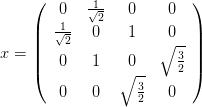 | (9.19) |
 | (9.20) |
 | (9.21) |
Our goal is to write a program that calculates the eigenvalues  of
the
  matrix
  . Instead of reinventing the wheel, we will use ready
made routines that calculate eigenvalues and eigenvectors of matrices found in the
Lapack library. This library can be found in the high quality numerical software
repository Netlib and more specifically at http://www.netlib.org/lapack/.
Documentation can be found at http://www.netlib.org/lapack/lug/, but it
is also easily accessible online by a Google search or by using the man
pages .
The programs have been written in the Fortran programming language, therefore
the reader should review the discussion in Section 6.1.2.
As inexperienced users we will first look for driver routines that perform a
diagonalization process. Since our task is to diagonalize a real symmetric matrix, we pick the
subroutine
DSYEV (D = double precision, SY = symmetric, EV = eigenvalues
with optional eigenvectors). If the documentation of the library is
installed in our system, we may use the Linux man pages for accessing
it:
> man dsyev
From this page we learn how to use this subroutine:
SUBROUTINE DSYEV( JOBZ, UPLO, N, A, LDA, W, WORK, LWORK, INFO )
CHARACTER JOBZ, UPLO
INTEGER INFO, LDA, LWORK, N
DOUBLE PRECISION A( LDA, * ),W( * ), WORK( * )
ARGUMENTS
JOBZ (input) CHARACTER*1
= ’N’: Compute eigenvalues only;
= ’V’: Compute eigenvalues and eigenvectors.
UPLO (input) CHARACTER*1
= ’U’: Upper triangle of A is stored;
= ’L’: Lower triangle of A is stored.
N (input) INTEGER
The order of the matrix A. N >= 0.
A (input/output) DOUBLE PRECISION array, dimension (LDA, N)
On entry, the symmetric matrix A. If UPLO = ’U’, the
leading N-by-N upper triangular part of A contains the
upper triangular part of the matrix A. If UPLO = ’L’,
the leading N-by-N lower triangular part of A contains
the lower triangular part of the matrix A. On exit, if
JOBZ = ’V’, then if INFO = 0, A contains
the orthonormal eigenvectors of the matrix A. If
JOBZ = ’N’, then on exit the lower triangle (if UPLO=’L’)
or the upper triangle (if UPLO=’U’) of A, including the
diagonal, is destroyed.
LDA (input) INTEGER
The leading dimension of the array A. LDA >= max(1,N).
W (output) DOUBLE PRECISION array, dimension (N)
If INFO = 0, the eigenvalues in ascending order.
WORK (workspace/output) DOUBLE PRECISION array, dimension
(LWORK).
On exit, if INFO = 0, WORK(1) returns the optimal LWORK.
LWORK (input) INTEGER
The length of the array WORK. LWORK >= max(1,3*N-1).
For optimal efficiency, LWORK >= (NB+2)*N, where NB is
the blocksize for DSYTRD returned by ILAENV.
If LWORK = -1, then a workspace query is assumed; the
routine only calculates the optimal size of the WORK
array, returns this value as the first entry of the
WORK array, and no error message related to LWORK is
issued by XERBLA.
INFO (output) INTEGER
= 0: successful exit
< 0: if INFO = -i, the i-th argument had an illegal value
> 0: if INFO = i, the algorithm failed to converge; i
off-diagonal elements of an intermediate tridiagonal
form did not converge to zero.
These originally cryptic pages contain all the necessary information and
the reader should familiarize herself with its format. For a quick and
dirty use of the routine, all we need to know is the types and usage of its
arguments. These are classified as “input”, “output” and “working space”
variables (some are in more than one classes). Input is the necessary data
that the routine needs in order to perform the computation. Output is
where the results of the computation are stored. And working space is the
memory provided by the user to the routine in order to store intermediate
results.
From the information above we learn that the matrix to be diagonalized is A
which is a rectangular matrix with the number of its rows and columns  .
The number of rows LDA (LDA= “leading dimension of A”) can be larger than
N is which case DSYEV will diagonalize the upper left N
 N part of the
matrix .
In our program we define a large matrix A[LDA][LDA] and diagonalize
a smaller submatrix A[N][N]. This way we can study many values of
 using the same matrix. The subroutine can be used in two ways:
- If JOBZ=’N’, it calculates only the eigenvalues of the matrix A[N][N]
and stores them in the array W[N], sorted in ascending order. We have
to be careful because, upon return, the routine destroys the lower
(UPLO=’U’) or upper (UPLO=’L’) triangular part of A. Be careful: the
documentation says the opposite, but I hope that you remember from
the discussion in Section 6.1.2 that Fortran arrays are transposed from
the point of view of C++! Since A is symmetric, only this part is needed
by DSYEV. If we need to reuse the matrix A, we have to make a backup
copy before the call to DSYEV.
- If JOBZ=’V’, it calculates both the eigenvalues and the eigenvectors
of the matrix A[N][N]. The eigenvalues are stored in the array W[N]
as before, whereas the corresponding eigenvectors in the columns
of the matrix A[N][N]. The eigenvectors are stored in the rows of
A[N][N], i.e. the n-th eigenvector corresponding to the eigenvalue
 W[n-1] is v=A[n-1]. The eigenvectors are normalized to unity,
i.e.
  v[m]*v[m]
 . The matrix A[N][N] is destroyed after
the call to DSYEV and if we need it we have to make a backup copy
before the call.
The reader should also familiarize herself with the use of the workspace array WORK.
This is memory space given to the routine for all its intermediate calculations.
Determining the size of this array needs some care. This is given by LWORK
and if performance is an issue the reader should read the documentation
carefully for its optimal determination. We will make the simple choice
LWORK=3*LDA-1. The variable INFO is used as a flag which informs the user
whether the calculation was successful, in which case its value is set to 0.
In our case, if INFO takes a non zero value, the program will abort the
calculation.
Before using the program in a complicated calculation, it is necessary to test
its use in a simple, easily controlled problem. We will familiarize ourselves with
the use of DSYEV by writing the following program:
#include <iostream>
#include <fstream>
#include <cstdlib>
#include <string>
#include <cmath>
using namespace std;
//--------------------------------------------------------
const int P = 100; //P=LDA
const int LWORK = 3*P-1;
double A[P][P], W[P], WORK[LWORK];
//--------------------------------------------------------
extern "C" void
dsyev_(const char& JOBZ,const char& UPLO,
const int & N,
double A[P][P],const int & LDA,
double W [P],
double WORK[P],
const int & LWORK, int & INFO);
//--------------------------------------------------------
int main(){
int N;
int i,j;
int LDA,INFO;
char JOBZ,UPLO;
string buf;
//Define the **symmetric** matrix to be diagonalized
//The subroutine uses the upper triangular part
//(UPLO=’U’) in the *FORTRAN* column-major mode,
//therefore in C++, we need to define its *lower*
//triangular part!
N = 4; // an N x N matrix
A[0][0]=-7.7;
A[1][0]= 2.1;A[1][1]= 8.3;
A[2][0]=-3.7;A[2][1]=-16.;A[2][2]=-12.;
A[3][0]= 4.4;A[3][1]= 4.6;A[3][2]=-1.04;A[3][3]=-3.7;
//We print the matrix A before calling DSYEV since
//it is destroyed after the call.
for(i=0;i<N;i++)
for(j=0;j<=i;j++)
cout << "A( " << i+1 << " , " << j+1 << " )="
<< A[i][j] << endl;
//We ask for eigenvalues AND eigenvectors (JOBZ=’V’)
JOBZ=’V’; UPLO=’U’;
cout << "COMPUTING WITH DSYEV:" << endl;
// LDA: Leading dimension of A = number of rows of
// full array
LDA = P;
dsyev_(JOBZ,UPLO,N,A,LDA,W,WORK,LWORK,INFO);
cout << "DSYEV: DONE. CHECKING NOW:" << endl;
if(INFO != 0){cerr << "DSYEV failed. INFO= "
<< INFO << endl;exit(1);}
//Print results: W(I) has the eigenvalues:
cout << "DSYEV: DONE.:" << endl;
cout << "EIGENVALUES OF MATRIX:" << endl;
cout.precision(17);
for(i=0;i<N;i++)
cout << "LAMBDA("<< i+1
<< ")=" << W[i] << endl;
//Eigenvectors are in stored in the rows of A:
cout << "EIGENVECTORS OF MATRIX:" << endl;
for(i=0;i<N;i++){
cout << "EIGENVECTOR " << i+1
<< " FOR EIGENVALUE " << W[i] << endl;
for(j=0;j<N;j++)
cout << "V_" << i+1 << "(" << j+1
<< ")= " << A[i][j] << endl;
}
}// main()
The next step is to compile and link the program. In order to link the program
to Lapack we have to instruct the linker ld where to find the libraries Lapack and
BLAS
and link them to our program. A library contains compiled software in archives of
object files. The convention for their names in a Unix environment is to start with
the string “lib” followed by the name of the library and a .a or .so extension.
For example, in our case the files we are interested in have the names
liblapack.so and libblas.so which can be searched in the file system by the
commands:
> locate libblas
> locate liblapack
In order to see the files that they contain we give the
commands :
> ar -t /usr/lib/libblas.so
> ar -t /usr/lib/liblapack.so
In the commands shown above you may have to substitute /usr/lib with the
path appropriate for your system. If the program is in the file test.cpp, the
compilation/linking command is:
> g++ test.cpp -o test -L/usr/lib -llapack -lblas
The option -L/usr/lib instructs the linker to look for libraries in the /usr/lib
directory ,
whereas the options -llapack -lblas instructs the linker to look for any
unresolved symbols (i.e. names of external functions and subroutines not coded in
our program) first in the library liblapack.a and then in the library
libblas.a.
The command shown above produces the executable file test which, when
run, produces the result:
EIGENVALUES OF MATRIX:
LAMBDA(1)=-21.411990695806409
LAMBDA(2)=-9.9339436575643028
LAMBDA(3)=-2.5576560809720039
LAMBDA(4)= 18.803590434342716
EIGENVECTORS OF MATRIX:
EIGENVECTOR 1 FOR EIGENVALUE -21.411990695806409
V_1(1)= -0.19784566233322534
V_1(2)= -0.4647986784623277
V_1(3)= -0.85469100929950759
V_1(4)= 0.1196769026094445
EIGENVECTOR 2 FOR EIGENVALUE -9.9339436575643028
V_2(1)= 0.82441241087467854
V_2(2)= -0.13242939824916203
V_2(3)= -0.19107651157591365
V_2(4)= -0.51603914386327754
EIGENVECTOR 3 FOR EIGENVALUE -2.5576560809720039
V_3(1)= 0.50268419698022238
V_3(2)= -0.24778437244453691
V_3(3)= 0.13285333709059657
V_3(4)= 0.81747262565942114
EIGENVECTOR 4 FOR EIGENVALUE 18.803590434342716
V_4(1)= 0.16884865648881003
V_4(2)= 0.83965918547426488
V_4(3)= -0.46405068276047351
V_4(4)= 0.22609632301334964
We are now ready to tackle the problem of computing the energy spectrum of the
anharmonic oscillator. The main program contains the user interface where the
basic parameters for the calculation are read from the stdin. The user can
specify the dimension DIM  of
of  and the coupling constant
  .
Then the program computes the eigenvalues
  of the
  matrix
  , which represents the action of the operator
  in the
 representation in
  . The tasks are allocated to the
subroutines calculate_X4, calculate_evs and calculate_H. The subroutine
calculate_X4 calculates the
  matrix
  . First, the matrix
  is
calculated and then
  is obtained by computing its fourth power. The
matrix
  can also be calculated analytically and this is left as an
exercise to the reader. The subroutine calculate_H calculates the matrix
 using the result for
  given by calculate_X4. Finally
the eigenvalues are calculated in the subroutine calculate_evs by a
call to DSYEV, which are returned to the main program for printing to
the stdout. The program is listed below and can be found in the file
anharmonic.cpp:
#include <iostream>
#include <fstream>
#include <cstdlib>
#include <string>
#include <cmath>
using namespace std;
//--------------------------------------------------------
const int P = 1000; //P=LDA
const int LWORK = 3*P-1;
int DIM;
double H[P][P], X[P][P], X4[P][P];
double E[P], WORK[LWORK];
double lambda;
//--------------------------------------------------------
extern "C" void
dsyev_(const char& JOBZ,const char& UPLO,
const int & N,
double H[P][P],const int & LDA,
double E [P],
double WORK[P],
const int & LWORK, int & INFO);
//--------------------------------------------------------
void calculate_X4 ();
void calculate_evs();
void calculate_H ();
//--------------------------------------------------------
int main(){
string buf;
cout << "# Enter Hilbert Space dimension:\n";
cin >> DIM; getline(cin,buf);
cout << "# Enter lambda:\n";
cin >> lambda; getline(cin,buf);
cout << "# lambda= " << lambda << endl;
cout << "# ########################################\n";
cout << "# Energy spectrum of anharmonic oscillator\n";
cout << "# using matrix methods.\n";
cout << "# Hilbert Space Dimension DIM = "<<DIM<< endl;
cout << "# lambda coupling = " << lambda << endl;
cout << "# ########################################\n";
cout << "# Output: DIM lambda E_0 E_1 .... E_{N-1} \n";
cout << "# ----------------------------------------\n";
cout.precision(15);
//Calculate X^4 operator:
calculate_X4();
//Calculate eigenvalues:
calculate_evs();
cout.precision(17);
cout << "EV " << DIM << " " << lambda << " ";
for(int n=0;n<DIM;n++) cout << E[n] << " ";
cout << endl;
}// main()
//--------------------------------------------------------
void calculate_evs(){
int INFO;
const char JOBZ=’V’,UPLO=’U’;
calculate_H();
dsyev_(JOBZ,UPLO,DIM,H,P,E,WORK,LWORK,INFO);
if(INFO != 0){
cerr << "dsyev failed. INFO= " << INFO << endl;
exit(1);
}
cout << "# ***************** EVEC *****************\n";
for( int n=0;n<DIM;n++){
cout << "# EVEC " << lambda << " ";
for(int m=0;m<DIM;m++)
cout << H[n][m] << " ";
cout << ’\n’;
}
}//calculate_evs()
//--------------------------------------------------------
void calculate_H(){
double X2[P][P];
for( int n =0;n<DIM;n++){
for(int m =0;m<DIM;m++)
H[n][m] = lambda*X4[n][m];
H [n][n]+= n+0.5;
}
cout << "# ***************** H *****************\n";
for(int n=0;n<DIM;n++){
cout << "# HH ";
for(int m=0;m<DIM;m++)
cout << H[n][m] << " ";
cout << ’\n’;
}
cout << "# ***************** H *****************\n";
}//calculate_H()
//--------------------------------------------------------
void calculate_X4(){
double X2[P][P];
const double isqrt2=1.0/sqrt(2.0);
for( int n=0;n<DIM;n++)
for(int m=0;m<DIM;m++)
X[n][m]=0.0;
for( int n=0;n<DIM;n++){
int m=n-1;
if(m>=0) X[n][m] = isqrt2*sqrt(double(m+1));
m =n+1;
if(m<DIM)X[n][m] = isqrt2*sqrt(double(m ));
}
// X2 = X . X
for( int n=0;n<DIM;n++)
for( int m=0;m<DIM;m++){
X2 [n][m] = 0.0;
for(int k=0;k<DIM;k++)
X2[n][m] += X [n][k]*X [k][m];
}
// X4 = X2 . X2
for( int n=0;n<DIM;n++)
for( int m=0;m<DIM;m++){
X4 [n][m] = 0.0;
for(int k=0;k<DIM;k++)
X4[n][m] += X2[n][k]*X2[k][m];
}
}//calculate_X4()
9.3 Results
Compiling and running the program can be done with the commands:
> g++ -O2 anharmonic.cpp -o an -llapack -lblas
> ./an
# Enter Hilbert Space dimension:
4
# Enter lambda:
0.0
.....
# ***************** H *****************
# HH 0.5 0 0 0
# HH 0 1.5 0 0
# HH 0 0 2.5 0
# HH 0 0 0 3.5
# ***************** H *****************
# ***************** EVEC *****************
# EVEC 0 1 0 0 0
# EVEC 0 0 1 0 0
# EVEC 0 0 0 1 0
# EVEC 0 0 0 0 1
EV 4 0 0.5 1.5 2.5 3.5
In the above program we used  and
and  . The
. The  choice leads us
to the simple harmonic oscillator and we obtain the expected solutions:
 ,
,  and the eigenstates (eigenvectors of
 )
)  . Similar results can be obtained for larger
 .
.
For non zero values of  , the finite
  calculation contains systematic errors
from neglecting all the matrix elements
  for
for  or
or  . Our
program calculates the eigenvalues
  of the finite matrix
  ,
,
 and one expects that
 | (9.22) |
where
 | (9.23) |
is the true  -th level eigenvalue of the Hamiltonian
  . In practice the limit
9.22 for given
  and
and  is calculated by computing
  numerically for
increasing values of
  . If convergence to a desired level of accuracy is achieved
for the accessible values of
  , then the approached limit is taken as an
approximation to
  . This process is shown graphically in figures 9.1-9.3 for
 . Convergence is satisfactory for quite small
  for
for  but
larger values of
  are needed for
  . Increasing the value of
  for fixed
 makes the use of larger values of
  necessary. Similarly for a given energy
level
  , increasing
  also makes the use of larger values of
  necessary. A
session that computes this limit for the ground level energy
  is shown
below :
> tcsh
> g++ -O2 anharmonic.cpp -llapack -lblas -o an
> foreach N (4 8 12 16 24 32)
foreach? (echo $N;echo 0.9) |./an >> data
foreach? end
> grep ^EV data | awk ’{print $2,$4}’
4 0.711467845686790
8 0.786328966767866
12 0.785237674919165
16 0.784964461939594
24 0.785032515135677
32 0.785031492177730
> gnuplot
gnuplot> plot "<grep ^EV data | awk ’{print 1/$2,$4}’"
Further automation of this process can be found in the shell script file
anharmonic.csh in the accompanying software. We note the large  convergence of
  and that we can take
  . For higher
accuracy, a computation using larger
  will be necessary.
We can also compute the expectation values  of an operator
 when the anharmonic oscillator is in a state
  :
:
 | (9.24) |
In practice, the expectation value will be computed from the limit
 | (9.25) |
where  are the eigenvectors of the finite
  matrix
  computed numerically by DSYEV. These are determined by their components
 , where
 | (9.26) |
which are stored in the columns of the array H after the call to DSYEV:
![cm (N, λ ) = H [n ][m ].](main_latex3328x.png) | (9.27) |
Substituting equation (9.26) to (9.24) we obtain
 | (9.28) |
and we can use (9.27) for the computation of the sum.
As an application, consider the expectation values of the operators  ,
,  and
and  . Taking into account that
 , we obtain the uncertainties


 and
and 
 . Their product
should satisfy Heisenberg’s uncertainty relation
  . The results are
shown in table 9.1 and in figures 9.4-9.5. The calculation is left as an exercise to
the reader.
The physics of the anharmonic oscillator can be better understood by studying
the large  limit. As shown in figure 9.5, the term
  dominates in this limit
and the expectation value
  decreases. This means that states that
confine the oscillator to a smaller range of
  are favored. This, using the
uncertainty principle, implies that the typical momentum of the oscillator
also increases in magnitude. This is confirmed in figure 9.5 where we
observe the expectation value
  to increase with
  . In order to
understand quantitatively these competing effects we will use a scaling
argument due to Symanzik. We redefine
  ,
,  in the
Hamiltonian
  and for large enough
  we
obtain
the asymptotic behavior
 | (9.29) |
where  is the Hamiltonian of the anharmonic “oscillator” with
 . Since the operator
  is independent of
  , the energy spectrum will
have the asymptotic behavior
 | (9.30) |
In reference [44] it is shown that for  we have that
 | (9.31) |
with an accuracy better than one part in  . For large values of
  , the authors
obtain the asymptotic behavior
 | (9.32) |
where 
 . This relation is tested
in figure 9.6 where we observe good agreement with our calculations.
Table 9.2: Numerical calculation of the energy levels of the anharmonic oscillator given
in reference [44].
|
|
|
|
|
|
 |  |  |  |  |  |
|
|
|
|
|
|
| 0.002 | 0.501 489 66 | 1.507 419 39 | 2.519 202 12 | 3.536 744 13 | 4.559 955 56 |
| 0.006 | 0.504 409 71 | 1.521 805 65 | 2.555 972 30 | 3.606 186 33 | 4.671 800 37 |
| 0.01 | 0.507 256 20 | 1.535 648 28 | 2.590 845 80 | 3.671 094 94 | 4.774 913 12 |
| 0.05 | 0.532 642 75 | 1.653 436 01 | 2.873 979 63 | 4.176 338 91 | 5.549 297 81 |
| 0.1 | 0.559 146 33 | 1.769 502 64 | 3.138 624 31 | 4.628 882 81 | 6.220 300 90 |
| 0.3 | 0.637 991 78 | 2.094 641 99 | 3.844 782 65 | 5.796 573 63 | 7.911 752 73 |
| 0.5 | 0.696 175 82 | 2.324 406 35 | 4.327 524 98 | 6.578 401 95 | 9.028 778 72 |
| 0.7 | 0.743 903 50 | 2.509 228 10 | 4.710 328 10 | 7.193 265 28 | 9.902 610 70 |
| 1 | 0.803 770 65 | 2.737 892 27 | 5.179 291 69 | 7.942 403 99 | 10.963 5831 |
| 2 | 0.951 568 47 | 3.292 867 82 | 6.303 880 57 | 9.727 323 19 | 13.481 2759 |
| 50 | 2.499 708 77 | 8.915 096 36 | 17.436 9921 | 27.192 6458 | 37.938 5022 |
| 200 | 3.930 931 34 | 14.059 2268 | 27.551 4347 | 43.005 2709 | 60.033 9933 |
| 1000 | 3.694 220 85 | 23.972 2061 | 47.017 3387 | 73.419 1140 | 102.516 157 |
| 8000 | 13.366 9076 | 47.890 7687 | 93.960 6046 | 146.745 512 | 204.922 711 |
| 20000 | 18.137 2291 | 64.986 6757 | 127.508 839 | 199.145 124 | 278.100 238 |
|
|
|
|
|
|
 |  |  |  |  | |
|
|
|
|
|
|
| 0.002 | 5.588 750 05 | 6.623 044 60 | 7.662 759 33 | 8.707 817 30 | |
| 0.006 | 5.752 230 87 | 6.846 948 47 | 7.955 470 29 | 9.077 353 66 | |
| 0.01 | 5.901 026 67 | 7.048 326 88 | 8.215 837 81 | 9.402 692 31 | |
| 0.05 | 6.984 963 10 | 8.477 397 34 | 10.021 9318 | 11.614 7761 | |
| 0.1 | 7.899 767 23 | 9.657 839 99 | 11.487 3156 | 13.378 9698 | |
| 0.3 | 10.166 4889 | 12.544 2587 | 15.032 7713 | 17.622 4482 | |
| 0.5 | 11.648 7207 | 14.417 6692 | 17.320 4242 | 20.345 1931 | |
| 0.7 | 12.803 9297 | 15.873 6836 | 19.094 5183 | 22.452 9996 | |
| 1 | 14.203 1394 | 17.634 0492 | 21.236 4362 | 24.994 9457 | |
| 2 | 17.514 1324 | 21.790 9564 | 26.286 1250 | 30.979 8830 | |
| 50 | 49.516 4187 | 61.820 3488 | 74.772 8290 | 88.314 3280 | |
| 200 | 78.385 6232 | 97.891 3315 | 118.427 830 | 139.900 400 | |
| 1000 | 133.876 891 | 167.212 258 | 202.311 200 | 239.011 580 | |
| 8000 | 267.628 498 | 334.284 478 | 404.468 350 | 477.855 700 | |
| 20000 | 363.201 843 | 453.664 875 | 548.916 140 | 648.515 330 | |
| |
|
|
|
|
|
|
9.4 The Double Well Potential
We can also use matrix methods in order to calculate the energy spectrum of a
particle in a double well potential given by the Hamiltonian:
 | (9.33) |
The equilibrium points of the classical motion are located at the minima:
 | (9.34) |
When the well is very deep, then for the lowest energy levels the potential can
be well approximated by that of a harmonic oscillator with angular frequency
 , therefore
 | (9.35) |
In this case the tunneling effect is very weak and the energy levels are arranged in
almost degenerate pairs. The corresponding eigenstates are symmetric and
antisymmetric linear combinations of states localized near the left and right
minima of the potential. For example, for the two lowest energy levels we expect
that
 | (9.36) |
where  and
and
 | (9.37) |
where the states  and
and  are localized to the left and right well of the
potential respectively (see also figure 10.4 of chapter 10).
We will use equations (9.12) in order to calculate the Hamiltonian (9.33) .
We need to make very small modifications to the code in the file anharmonic.cpp.
We will only add a routine that calculates the matrices  . The resulting
program can be found in the file doublewell.cpp:
//========================================================
// H : Hamiltonian operator H0+(lambda/4)*X^4
// H0 : Hamiltonian H0=1/2 P^2-1/2 X^2
// X,X2,X4: Position operator and its powers
// iP : i P operator
// P2 : P^2 = -(iP)(iP) operator
// E : Energy eigenvalues
// WORK : Workspace for lapack routine DSYEV
//========================================================
#include <iostream>
#include <fstream>
#include <cstdlib>
#include <string>
#include <cmath>
using namespace std;
//--------------------------------------------------------
const int P = 1000; //P=LDA
const int LWORK = 3*P-1;
int DIM;
double H [P][P], H0[P][P];
double X [P][P], X2[P][P], X4[P][P];
double iP[P][P], P2[P][P];
double E[P], WORK[LWORK];
double lambda;
//--------------------------------------------------------
extern "C" void
dsyev_(const char& JOBZ,const char& UPLO,
const int & N,
double H[P][P],const int & LDA,
double E [P],
double WORK[P],
const int & LWORK, int & INFO);
//--------------------------------------------------------
void calculate_ops();
void calculate_evs();
void calculate_H ();
//--------------------------------------------------------
int main(){
string buf;
cout << "# Enter Hilbert Space dimension:\n";
cin >> DIM; getline(cin,buf);
cout << "# Enter lambda:\n";
cin >> lambda; getline(cin,buf);
cout << "# lambda= " << lambda << endl;
cout << "# ########################################\n";
cout << "# Energy levels of double well potential \n";
cout << "# using matrix methods.\n";
cout << "# Hilbert Space Dimension DIM = "<<DIM<< endl;
cout << "# lambda coupling = " << lambda << endl;
cout << "# ########################################\n";
cout << "# Output: DIM lambda E_0 E_1 .... E_{N-1} \n";
cout << "# ----------------------------------------\n";
cout.precision(15);
//Calculate operators:
calculate_ops();
//Calculate eigenvalues:
calculate_evs();
cout.precision(17);
cout << "EV " << DIM << " " << lambda << " ";
for(int n=0;n<DIM;n++) cout << E[n] << " ";
cout << endl;
}// main()
//--------------------------------------------------------
void calculate_evs(){
int INFO;
const char JOBZ=’V’,UPLO=’U’;
calculate_H();
dsyev_(JOBZ,UPLO,DIM,H,P,E,WORK,LWORK,INFO);
if(INFO != 0){
cerr << "dsyev failed. INFO= " << INFO << endl;
exit(1);
}
cout << "# ***************** EVEC *****************\n";
for( int n=0;n<DIM;n++){
cout << "# EVEC " << lambda << " ";
for(int m=0;m<DIM;m++)
cout << H[n][m] << " ";
cout << ’\n’;
}
}//calculate_evs()
//--------------------------------------------------------
void calculate_H(){
double X2[P][P];
for( int n =0;n<DIM;n++)
for(int m =0;m<DIM;m++)
H[n][m] = H0[n][m] + 0.25*lambda*X4[n][m];
cout << "# ***************** H *****************\n";
for(int n=0;n<DIM;n++){
cout << "# HH ";
for(int m=0;m<DIM;m++)
cout << H[n][m] << " ";
cout << ’\n’;
}
cout << "# ***************** H *****************\n";
}//calculate_H()
//--------------------------------------------------------
void calculate_ops(){
double X2[P][P];
const double isqrt2=1.0/sqrt(2.0);
for( int n=0;n<DIM;n++)
for(int m=0;m<DIM;m++){
X[n][m]=0.0;iP[n][m]=0.0;
}
for( int n=0;n<DIM;n++){
int m=n-1;
if(m>=0 )X [n][m] = isqrt2*sqrt(double(m+1));
if(m>=0 )iP[n][m] = -isqrt2*sqrt(double(m+1));
m =n+1;
if(m<DIM)X [n][m] = isqrt2*sqrt(double(m ));
if(m<DIM)iP[n][m] = isqrt2*sqrt(double(m ));
}
// X2 = X . X
for( int n=0;n<DIM;n++)
for( int m=0;m<DIM;m++){
X2 [n][m] = 0.0;
for(int k=0;k<DIM;k++)
X2[n][m] += X [n][k]*X [k][m];
}
// X4 = X2 . X2
for( int n=0;n<DIM;n++)
for( int m=0;m<DIM;m++){
X4 [n][m] = 0.0;
for(int k=0;k<DIM;k++)
X4[n][m] += X2[n][k]*X2[k][m];
}
// P2 =-iP . iP
for( int n=0;n<DIM;n++)
for( int m=0;m<DIM;m++){
P2 [n][m] = 0.0;
for(int k=0;k<DIM;k++)
P2[n][m] -= iP[n][k]*iP[k][m];
}
// Hamiltonian:
for( int n=0;n<DIM;n++)
for( int m=0;m<DIM;m++)
H0[n][m] = 0.5*(P2[n][m]-X2[n][m]);
}//calculate_ops()
Where is the particle’s favorite place when it is in the states  and
and  ? The answer to this question is obtained from the study of the
expectation value of the position operator
  in each one of them. We know
that when the particle is in one of the energy eigenstates, then we have
that
 | (9.38) |
because the potential  is even. Therefore
where in the last line we used the relation (9.38) 
 and that the amplitudes
 .
Also
we have that
  . Therefore, if we have that
  and
and
 , we obtain
 | (9.40) |
Given that for finite  , the subroutine DSYEV returns approximations to the
coefficients
  in the columns of the matrix H[DIM][DIM] so that
  H[n][m], you may compare the value of
  with the classical values
 as
as  is increased.
9.5 Problems
- Calculate the matrix
 for
for  analytically. Calculate its
eigenvalues for
  . Compare your results with the numerical values
that you obtain from your program.
- Add the necessary code to the program in the file test.cpp so that it
checks that the eigenvectors satisfy their defining relations
 and that they form an orthonormal basis
  .
.
- Calculate
 and
and  for
for  with an accuracy better
than
  %.
%.
- For how large
 can you calculate
  for
for  with an accuracy
better than
  % when
  ?
?
- Calculate
 and
and  for
for  with step
  by
achieving accuracy better than
  %. How large should
  be taken
in each case?
- Calculate the expression that gives the matrix elements of the operator
 in the
  representation analytically. Modify the program in
anharmonic.cpp in order to incorporate your calculation. Verify that
the results are the same and test if it has an effect in the total
computation time with and without calculating the eigenvalues and
eigenvectors of the Hamiltonian. Compute in each case the dependence
of the cpu time on
  by computing the exponent (cpu time)
 for
for  .
.
- Modify the code in the file anharmonic.cpp so that the arrays H,
X, X4, E, WORK are dynamically allocated and their dimension is
determined by the variable DIM read by the program interactively.
- Make an attempt to reproduce the results of Hioe and Montroll [44]
given in table 9.2 for
 and
and  . What is the largest value of
 that you can study given your computational resources?
- Make an attempt to reproduce the results of Hioe and Montroll [44]
given by equation (9.31) . Calculate the ground state energy
 for
for
 and then fit your results to a function of the form
 . What is the accuracy in the calculation of
the coefficients
  ,
,  and
and  and how good is the agreement with
equation (9.31) ?
- Modify the code in the file anharmonic.cpp so that it calculates the
expectation values
 ,
,  and the corresponding
products
  .
.
(Hint: See the file anharmonicOBS.cpp.)
- Reproduce the results shown in figure 9.4. Repeat your calculation for
 . Repeat your calculations for
  .
.
- Reproduce the results shown in figure 9.5. Repeat your calculations for
 .
.
- Reproduce the results shown in figure 9.6. Repeat your calculation for
 .
.
- Write a program that calculates the energy levels of the anharmonic
oscillator
 | (9.41) |
Calculate  for
for  ,
,  and
and  .
.
- Modify the program of the previous problem so that it calculates the
expectation values
 ,
,  and the products
  .
Calculate the expectation values
  ,
,  and
and  for
for
 ,
,  and
and  .
.
- Use the program doublewell.cpp in order to calculate the energy
level pairs
 for
for  and
and  .
Calculate the difference
  and comment on your
results.
- Define the energy values
 Compare the results for
  of the previous problem with
 and
and  respectively. Explain your results.
- Modify the program doublewell.cpp, so that it calculates the expectation
values
 given by equation (9.40) . Compare
  with the
classical values
  for
for  .
.
- Repeat the previous problem when the states
 for
for  and
and  .
.
- For the simple harmonic oscillator, the energy levels are equidistant,
i.e.
 ,
,  . Calculate these
quantities for the anharmonic oscillator and the double well potential for
 and
and  . What do you conclude from your
results?
Chapter 10
Time Independent Schrödinger Equation
In this chapter, we will study the time independent Schrödinger equation
for a non relativistic particle of mass  , without spin, moving in one
dimension, in a static potential
  . We will only study bound states. The
solutions in this case yield the discrete energy spectrum
  as well as
the corresponding eigenstates of the Hamiltonian
  in position
representation.
From a numerical analysis point of view, the problem consists of solving for
the eigensystem of a differential equation with boundary conditions. Part of the
solution is the energy eigenvalue which also needs to be determined.
As an exercise, we will use two different methods, one that can be applied to a
particle in an infinite well with  , and one that can be applied to
more general cases. The first method is introduced only for educational
purposes and the reader may skip section 10.2 to go directly to section
10.3.
10.1 Introduction
The wave functions  , which are the position representation of the energy
eigenstates, satisfy the Schrödinger equation
 | (10.1) |
with the normalization condition
 | (10.2) |
The Hamiltonian operator is given in position representation by
 | (10.3) |
and it is Hermitian, i.e.  . Equation (10.1) is an eigenvalue
problem
 | (10.4) |
which, for bound states, has as solutions a discrete set of real functions
 such that
  . The numbers
  are real and they are the (bound) energy spectrum of the particle in the
potential
 . The minimum energy
  is called the ground state energy and the
corresponding ground state is given by a non trivial function
  . According to
the Heisenberg uncertainty principle, in this state the uncertainties in momentum
 and position
  so that
  .
.
The eigenstates  form an orthonormal basis
 | (10.5) |
so that any (square integrable) wave function  which represents the state
 is given by the linear combination
 | (10.6) |
The amplitudes 
 are complex numbers
that give the probability
  to measure energy
  in the state
 .
.
For any state  the function
 | (10.7) |
is the probability density of finding the particle at position  , i.e. the probability
of detecting the particle in the interval
 ![[x1,x2]](main_latex3560x.png) is given by
is given by
 | (10.8) |
The normalization condition (10.2) reflects the conservation of probability
(independent of time, respected by the time dependent Schrödinger equation) and
the completeness (in this case the certainty that the particle will be observed
somewhere on the  axis).
The classical observables  of this quantum mechanical system are
functions of the position and the momentum and their quantum mechanical
versions are given by operators
  . Their expectation values when the
system in a state
  are given by
 | (10.9) |
From a numerical point of view, the eigenvalue problem (10.1) requires the
solution of an ordinary second order differential equation. There are certain
differences in this problem compared to the ones studied in previous sections:
- Instead of an initial value problem (i.e. the values of the function and its
derivative are given at one point), we have a boundary value problem
(values of the function or its derivative given at two different points).
- The eigenvalue (energy) is unknown and should be determined as part
of the solution.
As an introduction to such classes of problems, we will present some simple methods
which are special to one dimension.
For the numerical solution of the above equation we renormalize  , the
function
  and the parameters so that we deal only with dimensionless
quantities. Equation (10.1) is rewritten as:
 | (10.10) |
Then we choose a length scale  which is defined by the parameters of the
problem
and we redefine
  . We define
 and we obtain
 | (10.11) |
We define 
 ,
,  and
change notation to
  ,
,  . We obtain
 | (10.12) |
The solutions of equation (10.1) can be obtained from those of equation (10.12) by using the
following “dictionary” :
 | (10.13) |
The dimensionless momentum is defined as 
 and we
obtain
 | (10.14) |
The commutation relation ![[x, p] = iℏ](main_latex3593x.png) becomes
becomes ![[˜x, ˜p] = i](main_latex3594x.png) . The kinetic energy
. The kinetic energy
 is given by
 | (10.15) |
and the Hamiltonian 
 | (10.16) |
In what follows, we will omit the tilde above the symbols and write  instead of
 .
.
10.2 The Infinite Potential Well
The simplest model for studying the qualitative features of bound states is the
infinite potential well of width  where a particle is confined within the interval
![[− L∕2,L ∕2]](main_latex3602x.png) :
:
 | (10.17) |
The length scale chosen here is  and the dimensionless variable
  corresponds to
  when
when  is measured in length units.
The solution of (10.12) can be easily computed. Due to the symmetry
 | (10.18) |
of the potential, the solutions have well defined parity. This property will be
crucial to the method used below. The method discussed in the next section can
also be used on non even potentials.
The solutions are divided into two categories, one with even parity

 for
for  and one with odd parity

 for
for  .
.
 | (10.19) |
where
 | (10.20) |
and the normalization has been chosen so
that
 .
.
The solutions can be found by using the parity of the wave functions. We note
that for the positive parity solutions
 | (10.21) |
whereas for the negative parity solutions
 | (10.22) |
The constant  depends on the normalization of the wave function. Therefore
we can set
  originally and then renormalize the wave function so
that equation (10.2) is satisfied. If the energy is known, the relations
(10.21) and (10.22) can be taken as initial conditions in relation (10.12) .
By using a Runge–Kutta algorithm we can evolve the solution towards
 . The problem is that the energy
  is unknown. If the energy
is not allowed by the quantum theory we will find that the boundary
conditions
 | (10.23) |
are violated. As we approach the correct value of the energy, we obtain
 .
.
Therefore we follow the steps described below:
- We choose an initial value for the energy
 that is lower than the
one we are looking for. We can use estimates from known solutions
of similar looking potential wells or simply start from a value slightly
higher than the absolute minimum of the potential.
- We choose the parity of the solution and we set initial conditions
according to equations (10.21) and (10.22) .
- We evolve the solutions using a 4th order Runge-Kutta method from
 to
to  .
.
- If equation (10.23) is not satisfied, we increase the energy by
 and
we repeat.
- We repeat until
 changes sign. Then we lower the energy by
 .
.
- The process is ended when
 for appropriately chosen
small
  .
.
For the evolution of the solution from  to
to  we use the 4th order
Runge-Kutta method programmed in the file rk.cpp of chapter 4. We copy the
function RKSTEP in a local file rk.cpp. The integration of (10.12) can by done by
using the function
with the initial conditions We use the notation  psi,
psi,  psip. The functions f1 and f2
correspond to the right hand side of (10.24) . They are the derivatives of
 and
and  respectively and f1=psip, f2=(V-energy)*psi. The
code of f1 and f2 is put in a different file so that we can easily reuse
the code for many different potentials
  . The file wellInfSq.cpp
contains the necessary program for the potential of equation (10.17)
:
//===========================================================
//file: wellInfSq.cpp
//
//Functions used in RKSTEP function. Here:
//f1 = psip(x) = psi(x)’
//f2 = psip(x)’= psi(x)’’
//
//All one has to set is V, the potential
//===========================================================
#include <iostream>
#include <fstream>
#include <cstdlib>
#include <string>
#include <cmath>
using namespace std;
extern double energy;
//-------- trivial function: derivative of psi
double
f1(const double& x, const double& psi,const double& psip){
return psip;
}
//===========================================================
//-------- the second derivative of wavefunction:
//psip(x)’ = psi(x)’’ = -(E-V) psi(x)
double
f2(const double& x, const double& psi,const double& psip){
double V;
//------- potential, set here:
V = 0.0;
//------- Schroedinger eq: RHS
return (V-energy)*psi;
}
We stress that the energy  energy is put in the global scope so that it can
be accessed by the main program.
The main program is in the file well.cpp. The user enters the parameters
(energy, parity, Nx) and the loop
while(iter < 10000){
....
if(abs(psinew) <= epsilon) break;
if(psinew*psiold < 0.0 ) de = -0.5*de;
energy += de;
....
}
exits when  psinew has an absolute value which is less than epsilon, i.e.
when the condition (10.23) is satisfied to the desired accuracy. The value of the
energy increases up to the point where the sign of the wave function at
  changes (psinew*psiold
 ). Then the value of the energy is overestimated
and we change the sign of the step de and reduce its magnitude by a half. The
algorithm described on page 1072 is implemented inside the loop. After exiting
the loop, the energy has been determined with the desired accuracy and the rest
of the program stores the solution in the array psifinal(STEPS). The results
are written to the file psi.dat. Note how the variable parity is used so
that both cases parity
 can be studied. The full program is listed
below:
//===========================================================
//file: well.cpp
//
//Computation of energy eigenvalues and eigenfunctions
//of a particle in an infinite well with V(-x)=V(x)
//
//Input: energy: initial guess for energy
// parity: desired parity of solution (+/- 1)
// Nx-1 : Number of RK4 steps from x=0 to x=1
//Output: energy: energy eigenvalue
// psi.dat: final psi[x]
// all.dat: all psi[x] for trial energies
//===========================================================
#include <iostream>
#include <fstream>
#include <cstdlib>
#include <string>
#include <cmath>
using namespace std;
//--------------------------------------------------------
const int P = 10000;
double energy;
//--------------------------------------------------------
void
RKSTEP( double& t, double& x1,
double& x2,
const double& dt);
//--------------------------------------------------------
int main(){
double dx,x,epsilon,de;
double psi,psip,psinew,psiold;
double array_psifinal[2*P+1],array_xstep[2*P+1];
double *psifinal = array_psifinal+P;
double *xstep = array_xstep +P;
//psifinal points to (array_psifinal+P) and one can
//use psifinal[-P]...psifinal[P]. Similarly for xstep
int parity,Nx,iter,i,node;
string buf;
//------ Input:
cout << "Enter energy,parity,Nx:\n";
cin >> energy >> parity >> Nx; getline(cin,buf);
if(Nx > P){cerr << "Nx>P\n";exit(1);}
if(parity > 0) parity= 1;
else parity=-1;
cout << "# #######################################\n";
cout << "# Estart= " << energy
<< " parity= " << parity << endl;
dx = 1.0/(Nx-1);
epsilon = 1.0e-6;
cout << "# Nx= " << Nx << " dx = " << dx
<< " eps= " << epsilon << endl;
cout << "# #######################################\n";
//------ Calculate:
ofstream myfile("all.dat");
myfile.precision(17);
cout .precision(17);
iter = 0;
psiold = 0.0;
psinew = 1.0;
de = 0.1 * abs(energy);
while(iter < 10000){
// Initial conditions at x=0
x = 0.0;
if(parity == 1){
psi = 1.0;
psip = 0.0;
}else{
psi = 0.0;
psip = 1.0;
}
myfile << iter << " " << energy << " "
<< x << " " << psi << " "
<< psip << endl;
// Use Runge-Kutta to forward to x=1
for(i=2;i<=Nx;i++){
x = (i-2)*dx;
RKSTEP(x,psi,psip,dx);
myfile << iter << " " << energy << " "
<< x << " " << psi << " "
<< psip << endl;
}
psinew = psi;
cout << iter << " " << energy << " "
<< de << " " << psinew << endl;
// Stop if value of psi close to 0
if(abs(psinew) <= epsilon) break;
// Change direction of energy search:
if(psinew*psiold < 0.0 ) de = -0.5*de;
energy += de;
psiold = psinew;
iter++;
}//while(iter < 10000)
myfile.close();
//We found the solution:
//calculate it once again and store it
if(parity == 1){
psi = 1.0;
psip = 0.0;
node = 0; //count number of nodes of function
}else{
psi = 0.0;
psip = 1.0;
node = 1;
}
x = 0.0;
xstep [0] = x;
psifinal[0] = psi; //array that stores psi(x)
psiold = 0.0;
// Use Runge-Kutta to move to x=1
for(i=2 ; i<=Nx ; i++ ){
x = (i-2)*dx;
RKSTEP(x,psi,psip,dx);
xstep [i-1] = x;
psifinal[i-1] = psi;
// Use parity to compute psi(-x)
xstep [1-i] = -x;
psifinal[1-i] = psi*parity;
// Determine zeroes of psi(x):
// psi should not be zero within epsilon:
if(abs(psi) > 2.0*epsilon){
if(psi*psiold < 0.0) node += 2;
psiold = psi;
}
}//for(i=2;i<=Nx;i++)
node++;
//print final solution:
myfile.open("psi.dat");
cout << "Final result: E= " << energy
<< " n= " << node
<< " parity= " << parity << endl;
myfile << "# E= " << energy
<< " n= " << node
<< " parity= " << parity << endl;
for(i=-(Nx-1);i<=(Nx-1);i++)
myfile << xstep [i] << " "
<< psifinal[i] << endl;
myfile.close();
}// main()
The compilation and running of the program can be done with the commands
> g++ well.cpp wellInfSq.cpp rk.cpp -o well
> ./well
Enter energy,parity,Nx:
2.0 1 400
# #######################################
# Estart= 2 parity= 1
# Nx= 400 dx = 0.00250627 eps= 1e-06
# #######################################
0 2 0.200000000 0.155943694
1 2.2000000000 0.200000000 0.087444801
.....
28 2.4674072265 1.220703125e-05 -1.950054368e-06
29 2.4674011230 -6.103515625e-06 -7.246215909e-09
Final result: E= 2.4674011230468746 n= 1 parity= 1
The energy is determined to be  2.467401123 which can be compared to the
exact value
  2.467401100. The fractional error is
  . The
convergence can be studied graphically in figure 10.2.
The calculation of the excited states is done by changing the parity and by
choosing the initial energy slightly higher than the one determined in the previous
step .
The results are in table 10.1. The agreement with the exact result  is excellent.
We close this section with two more examples. First, we study a potential well
with triangular shape at its bottom
 | (10.26) |
and then a double well potential with
 | (10.27) |
where the parameters  are positive numbers. A qualitative plot of these
functions is shown in figure 10.1.
For the triangular potential we take  , whereas for the double well
potential
  and
and  . The code in wellInfSq.cpp is appropriately
modified and saved in the files wellInfTr.cpp and wellInfDbl.cpp respectively.
All we have to do is to change the line computing the value of the potential in the
function f2. For example the file wellInfTr.cpp contains the code
//------- potential, set here:
V = 10.0 * abs(x);
whereas the file wellInfDbl.cpp contains the code
//------- potential, set here:
if(abs(x) <= 0.3)
V = 100.0;
else
V = 0.0;
The analysis is performed in exactly the same way and the results are shown in
table 10.1. Note that, for large enough  , the energy levels of all the potentials
that we studied above tend to have identical values. This happens because, when
the particle has energy much larger than
  , the details of the potential at the
bottom do not influence its dynamical properties very much. For the triangular
potential, the energy levels have higher values than the corresponding ones of the
square potential. This happens because, on the average, the potential energy is
higher and the potential tends to confine the particle to a smaller region (
 is
decreased, therefore
  is increased). This can be seen in figure 10.3
where the wave functions of the particle in each of the two potentials are
compared.
Similar observations can be made for the double well potential. Moreover, we
note the approximately degenerate energy levels, something which is expected for
potentials of this form. This can be understood in terms of the localized
states given by the wave functions  and
and
 . The first one represents a state where
the particle is localized in the left well and the second one in the right.
This is shown in figure 10.4. As
  the two wells decouple and
the wave functions
  become equal to the energy eigenstate wave
functions of two particles in separate infinite square wells of width
  with energy eigenvalues
  . The difference of
  and
and  from these two values is due to the finite
  (see problem 4).
We will now discuss the limitations of this method. First, the method can be
used only on potential wells that are even, i.e.  . We used this
assumption in equations (10.21) and (10.22) giving the initial conditions for
states of well defined parity. When the potential is even, the energy eigenstates
have definite parity. The other problem can be understood by solving problem 4:
When
  , the wave function is almost zero around
  and
the integration from
  to
to  will be dominated by numerical
errors. The same is true when the particle has to go through high potential
barriers.
This method can also we used on potential wells that are not infinite. In that
case we can add infinite walls at points that are far enough so that the wave
function is practically zero there. Then the influence of this artificial wall will be
negligible (see problem 3).
10.3 Bound States
A serious problem with the method discussed in the previous section is that it
is numerically unstable. You should have already realized that if you tried to solve
problem 3. In that problem, when the walls are moved further than  , the
convergence of the algorithm becomes harder. You can understand this by
realizing that in the integration process the solution is evolved from the classically
allowed into the classically forbidden region so that an oscillating solution
changes into an exponentially damped one. But as
  there are two
solutions, one that is physically acceptable
  and one that is
diverging
  which is not acceptable due to (10.2) . Therefore, in
order to achieve convergence to the physically acceptable solution, the
energy has to be finely tuned, especially when we integrate towards large
 . For this reason it is preferable to integrate from the exponentially
damped region towards the oscillating region. The idea is to start integrating
from these regions and try to match the solutions and their derivatives at
appropriately chosen matching points. The matching is achieved at a
point
  by trying to determine the value of the energy that sets the
ratio
 | (10.28) |
equal to zero, within the attainable numerical accuracy. It is desirable to
choose a point  within the classical region (
 ) and usually
we pick a turning point
  . By renormalizing
  we can
always set
  , therefore
  means that
 . The denominator of (10.28) sets the scale of the desired
accuracy
The idea is depicted in figure 10.5. The algorithm is the following:
- Choose the integration interval [xmin,xmax].
- Choose the initial conditions
 ,
,  ,
,
 ,
,  . This choice depends on the potential
 . Usually we take xmin and xmax deep enough in the classically
forbidden region and choose the values
  ,
,  to
be zero or exponentially small (e.g.
  ,
,  ). The
corresponding values of the derivatives
  ,
,  are also taken to be small. The arbitrary normalization of
  allows
these initial values to be chosen in a crude way. The relative sign of
the derivatives at large
  (determined e.g. by the parity of the wave
function for even potentials) is also taken care by the renormalization
of
  when applying the matching condition. For an infinite well,
the points xmin,xmax are the ones where the potential becomes infinite
and
  .
.
- Choose the initial value of the energy
 and of the energy variation
step
  .
.
- Calculate xm from the initial value of the energy and the solution of
 . Choose the solution that is at the left most side .
- Evolve the equations (10.24) from xmin to xm and obtain the solutions
 ,
, .
.
- Evolve the equations (10.24) from xmax to xm and obtain the solutions
 ,
, .
.
- Renormalize
 , so that
 .
.
- Compute the ratio
 of equation (10.28) .
- If
 for appropriately chosen
  , the calculation ends.
The result for the energy eigenvalue and eigenfunction is considered to
be determined with adequate accuracy and we may proceed with the
analysis of the results.
- If
 changes sign it means that we have crossed the energy
eigenvalue. Reverse the direction of search by taking
  .
.
- Change the energy
 and repeat by going back to the fourth
step.
When we exit the above loop, the current wave function is a good approximation to
the eigenfunction  corresponding to the eigenvalue
  . We normalize the
wave function according to equation (10.2) and we calculate the expectation
values according to (10.9) . It is also interesting to determine the number of
nodes
 of the wave function which is related to
  by
by  .
.
Our program needs to implement the Runge–Kutta algorithm. We use the
function RKSTEP (see page 525) which performs a 4th order Runge–Kutta step. Its
code is copied to the file rk.cpp.
The potential  is coded in the function V(x). The boundary conditions
are programmed in the function boundary(xmin, xmax, psixmin, psipxmin,
psixmax, psipxmax) which returns the values of psixmin =
  ,
psipxmin =
  , psixmax =
  , psipxmax =
  to the calling program. These functions are put in a separate file for each
potential that we want to study. The name of the file is related to the form
of the potential, e.g. we choose schInfSq.cpp for the infinite potential
well of (10.17) . The same file contains the code for the functions f1,
f2:
//===========================================================
//file: schInfSq.cpp
//===========================================================
//----- potential:
#include <iostream>
#include <fstream>
#include <cstdlib>
#include <string>
#include <cmath>
using namespace std;
extern double energy;
//--------
double V (const double& x ){
return 0.0;
}//V()
//-------- boundary conditions:
void
boundary (const double& xmin,const double& xmax ,
double& psixmin, double& psipxmin,
double& psixmax, double& psipxmax){
//for infinite square well we set psi=0 at boundary
//and psip=+/-1
psixmin = 0.0;
psipxmin = 1.0;
psixmax = 0.0;
psipxmax = -1.0;
//Initial values at xmin and xmax
}
//-------- trivial function: derivative of psi
double
f1(const double& x, const double& psi,const double& psip){
return psip;
}
//-------- the second derivative of wavefunction:
//psip(x)’ = psi(x)’’ = -(E-V) psi(x)
double
f2(const double& x, const double& psi,const double& psip){
//------- Schroedinger eq: RHS
return (V(x)-energy)*psi;
}
We note that if the potential becomes infinite for  xmin and/or
  xmax,
then this will be determined by the boundary conditions at xmin and/or
xmax.
The main program is in the file sch.cpp. The code is listed below and it
includes the function integrate(psi, dx, Nx) used for the normalization
of the wave function. It performs a numerical integration of the square
of a function whose values psi[i] i=0,...,Nx-1 are given at an odd
number of Nx equally spaced points by a distance dx using Simpson’s
rule.
//===========================================================
//
// File: sch.cpp
//
// Integrate 1d Schrodinger equation from xmin to xmax.
// Determine energy eigenvalue and eigenfunction by matching
// evolving solutions from xmin and from xmax at a point xm.
// Mathing done by equating values of functions and their
// derivatives at xm. The point xm chosen at the left most
// turning point of the potential at any given value of the
// energy. The potential and boundary conditions chosen in
// different file.
// ----------------------------------------------------------
// Input: energy: Trial value of energy
// de: energy step, if matching fails de -> e+de, if
// logderivative changes sign de -> -de/2
// xmin, xmax, Nx
// ----------------------------------------------------------
// Output: Final value of energy, number of nodes of
// wavefunction in stdout
// Final eigenfunction in file psi.dat
// All trial functions and energies in file all.dat
//===========================================================
#include <iostream>
#include <fstream>
#include <cstdlib>
#include <string>
#include <cmath>
using namespace std;
//--------------------------------------------------------
const int P = 20001;
double energy;
//--------------------------------------------------------
double V (const double& x );
double integrate(double* psi ,
const double& dx ,const int & Nx );
void
boundary (const double& xmin,const double& xmax ,
double& psixmin, double& psipxmin,
double& psixmax, double& psipxmax);
void
RKSTEP( double& t , double& x1,
double& x2 ,
const double& dt );
//--------------------------------------------------------
int main(){
int Nx,NxL,NxR;
double psi[P],psip[P];
double dx;
double xmin,xmax,xm; //left/right/matching points
double psixmin ,psipxmin ,psixmax ,psipxmax;
double psileft ,psiright ,psistep ,psinorm;
double psipleft,psipright,psipstep;
double de,epsilon;
double matchlogd,matchold,psiold,norm,x;
int iter,i,imatch,nodes;
string buf;
//Input:
cout << "# Enter energy,de,xmin,xmax,Nx:\n";
cin >> energy>>de>>xmin>>xmax>>Nx;getline(cin,buf);
//need even intervals for normalization integration:
if(Nx %2 == 0) Nx++;
if(Nx >P ){cerr << "Error: Nx > P \n";exit(1);}
if(xmin>=xmax){cerr << "Error: xmin>=xmax\n";exit(1);}
dx = (xmax-xmin)/(Nx-1);
epsilon = 1.0e-6;
boundary(xmin,xmax,psixmin,psipxmin,psixmax,psipxmax);
cout <<"# #######################################\n";
cout <<"# Estart= "<< energy <<" de= "<< de << "\n";
cout <<"# Nx= " << Nx <<" eps= " << epsilon << "\n";
cout <<"# xmin= "<< xmin << "xmax= "<< xmax
<<" dx= " << dx << "\n";
cout <<"# psi(xmin)= "<< psixmin
<<" psip(xmin)= "<< psipxmin << "\n";
cout <<"# psi(xmax)= "<< psixmax
<<" psip(xmax)= "<< psipxmax << "\n";
cout <<"# #######################################\n";
//Calculate:
ofstream myfile("all.dat");
myfile.precision(17);
cout .precision(17);
matchold = 0.0;
for(iter=1;iter<=10000;iter++){
//Determine matching point at turning point from the left:
imatch=-1;
for(i=0;i<Nx;i++){
x = xmin + i * dx;
if(imatch < 0 && (energy-V(x)) > 0.0) imatch = i;
}
if(imatch < 100 || imatch >= Nx-100) imatch = Nx/5-1;
xm = xmin + imatch*dx;
NxL = imatch+1;
NxR = Nx-imatch;
//Evolve wavefunction from the left:
psi [0] = psixmin;
psip [0] = psipxmin;
psistep = psixmin;
psipstep = psipxmin;
for(i=1;i<NxL;i++){
x = xmin+(i-1)*dx;//this is x before the step
RKSTEP(x,psistep,psipstep, dx);
psi [i] = psistep;
psip[i] = psipstep;
}
//use this to normalize eigenfunction to match at xm
psinorm = psistep;
psipleft = psipstep;
//Evolve wavefunction from the right:
psi [Nx-1]= psixmax;
psip[Nx-1]= psipxmax;
psistep = psixmax;
psipstep = psipxmax;
for(i=1;i<NxR;i++){
x = xmax-(i-1)*dx;
RKSTEP(x,psistep,psipstep,-dx);
psi [Nx-i-1] = psistep;
psip[Nx-i-1] = psipstep;
}
psinorm = psistep/psinorm;
psipright = psipstep;
//Renormalize psil so that psil(xm)=psir(xm)
for(i=0;i<NxL-1;i++){
psi [i] *= psinorm;
psip[i] *= psinorm;
}
psipleft *= psinorm;
//print current solution:
for(i=0;i<Nx;i++){
x = xmin + i *dx;
myfile << iter <<" "<<energy<<" "
<< x <<" "<<psi[i]<<" "
<<psip[i] <<"\n";
}
//matching using derivatives:
//Careful: this can fail if psi’(xm) = 0
//(use also |de|<1e-6 criterion)
matchlogd =
(psipright-psipleft)/(abs(psipright)+abs(psipleft));
cout << "# iter,energy,de,xm,logd: "
<< iter << " "
<< energy << " "
<< de << " "
<< xm << " "
<< matchlogd << "\n";
//break condition:
if(abs(matchlogd)<=epsilon ||
abs(de/energy)< 1.0e-12 ) break;
if(matchlogd * matchold < 0.0 ) de = -0.5*de;
energy += de;
matchold = matchlogd;
}//for(iter=1;iter<=10000;iter++)
myfile.close();
//------------------------------------------------------
//Solution has been found and now it is stored:
norm = integrate(psi,dx,Nx);
norm = 1.0/sqrt(norm);
//for(i=0;i<Nx;i++) psi[i] *= norm;
//Count number of zeroes, add one and get energy level:
nodes = 1;
psiold = psi[0];
for(i=1;i<Nx-1;i++)
if(abs(psi[i]) > epsilon){
if(psiold*psi[i] < 0.0 ) nodes++;
psiold = psi[i];
}
//Print final solution:
myfile.open("psi.dat");
cout << "Final result: E= " << energy
<< " n= " << nodes
<< " norm= " << norm << endl;
if(abs(matchlogd) > epsilon)
cout << "Final result: SOS: logd>epsilon. logd= "
<< matchlogd << endl;
myfile << "# E= " << energy
<< " n= " << nodes
<< " norm = " << norm << endl;
for(i=0;i<Nx;i++){
x = xmin + i * dx;
myfile << x << " " << psi[i] << "\n";
}
myfile.close();
}//main()
//========================================================
//Simpson’s rule to integrate psi(x)*psi(x) for proper
//normalization. For n intervals of width dx (n even)
//Simpson’s rule is:
//int(f(x)dx) =
//(dx/3)*(f(x_0)+4 f(x_1)+2 f(x_2)+...+4 f(x_{n-1})+f(x_n))
//
//Input: Discrete values of function psi[Nx], Nx is odd
// Integration step dx
//Returns: Integral(psi(x)psi(x) dx)
//========================================================
double integrate(double* psi,
const double& dx ,const int& Nx){
double Integral;
int i;
//zeroth order point:
i = 0;
Integral = psi[i]*psi[i];
//odd order points:
for(i=1;i<=Nx-2;i+=2) Integral += 4.0*psi[i]*psi[i];
//even order points:
for(i=2;i<=Nx-3;i+=2) Integral += 2.0*psi[i]*psi[i];
//last point:
i = Nx-1;
Integral += psi[i]*psi[i];
//measure normalization:
Integral *=dx/3.0;
return Integral;
}//integrate()
The reproduction of the results of the previous section for the infinite potential
well is left as an exercise. The compilation and running of the program can be
done with the commands:
> g++ sch.cpp schInfSq.cpp rk.cpp -o s
> ./s
# Enter energy,de,xmin,xmax,Nx:
1 0.5 -1 1 2000
# #######################################
# Estart= 1 de= 0.5
# Nx= 2001 eps= 1e-06
# xmin= -1 xmax= 1 dx= 0.001
# psi(xmin)= 0 psip(xmin)= 1
# psi(xmax)= 0 psip(xmax)= -1
# #######################################
# iter,energy,de,xm,logd: 1 1.0000 0.500 -0.601 -0.9748
# iter,energy,de,xm,logd: 2 1.5000 0.500 -0.601 -0.6412
.....
# iter,energy,de,xm,logd: 30 2.4674 -3.815E-6 -0.601 -1.0E-6
# iter,energy,de,xm,logd: 31 2.4674 1.907E-6 -0.601 2.7E-7
Final result: E= 2.467401504516602 n= 1 norm = 1.5707965025
We set xmin= -1, xmax = 1, Nx= 2000 and  ,
,  . The energy of
the ground state is found to be
  . The wave
function is stored in the file psi.dat and can be plotted with the gnuplot
command
gnuplot> plot "psi.dat" using 1:2 with lines
The functions computed during the iterations of the algorithm are stored in
the file all.dat. The first column is the iteration number (here we have iter =
0, ... 31) and we can easily filter each one of them with the commands
gnuplot> plot "<awk ’$1==1’ all.dat" using 3:4 w l t "iter=1"
gnuplot> replot "<awk ’$1==2’ all.dat" using 3:4 w l t "iter=2"
gnuplot> replot "<awk ’$1==3’ all.dat" using 3:4 w l t "iter=3"
gnuplot> replot "<awk ’$1==4’ all.dat" using 3:4 w l t "iter=4"
.....
which reproduce figure 10.6.
10.4 Measurements
The action of an operator  on a state
  can be easily calculated in the
position representation by its action on the corresponding wave function
  .
The action of the operators
 | (10.29) |
yield
 | (10.30) |
Using equation (10.9) we can calculate the expectation value  of the
operator
  when the system is at the state
  . Interesting examples are the
observables “position”
  , “position squared”
  , “momentum”
  , “momentum
squared”
  , “kinetic energy”
  , “potential energy”
  , “energy” or
“Hamiltonian”
  whose expectation values are given by the relations
We remind the reader that we used the dimensionless  as well as
equations (10.15) and (10.16) . Especially interesting are the “uncertainties”
 ,
,  that satisfy the inequality (“Heisenberg’s
uncertainty relation”)
 | (10.32) |
In the previous section we described how to calculate numerically the
eigenfunctions of the Hamiltonian. If  , we obtain that
 . Other operators need a numerical approximation
for the calculation of their expectation values. If the values of the wave
function are given at
  equally spaced points
  , then we
obtain
 | (10.33) |
where  and
and
 | (10.34) |
Both equations entail an error of the order of  . Special care should be taken at
the endpoints of the interval
 ![[x ,x ]
1 N](main_latex3811x.png) . As a first approach we will use the naive
approximations
. As a first approach we will use the naive
approximations
and The relevant program that calculates  ,
,  ,
,  ,
,  ,
,  ,
,  can be
found in the file observables.cpp and is listed below:
//===========================================================
//
// File observables.cpp
// Compile: g++ observables.cpp -o o
// Usage: ./o <psi.dat>
//
// Read in a file with a wavefunction in the format of psi.dat:
// # E= <energy> ....
// x1 psi(x1)
// x2 psi(x2)
// ............
//
// Outputs expectation values:
// normalization Energy <x> <p> <x^2> <p^2> Dx Dp DxDp
// where Dx = sqrt(<x^2>-<x>^2) Dp = sqrt(<p^2>-<p>^2)
// DxDp = Dx * Dp
//
//===========================================================
#include <iostream>
#include <fstream>
#include <cstdlib>
#include <string>
#include <cmath>
using namespace std;
//--------------------------------------------------------
double integrate(double* psi ,
const double& dx ,const int & Nx );
//--------------------------------------------------------
int main(int argc, char **argv){
const int P = 50000;
int Nx,i;
double xstep[P],psi[P],obs[P];
double xav, pav, x2av, p2av, Dx, Dp, DxDp,energy,h,norm;
string buf;
char *psifile;
if(argc != 2){
cerr << "Usage: " << argv[0] << " <filename>\n";
exit(1);
}
psifile = argv[1];
ifstream ifile(psifile);
if(! ifile){
cerr << "Error reading from file " << psifile << endl;
exit(1);
}
cout << "# reading wavefunction from file: "
<< psifile << endl;
ifile >> buf >> buf >> energy; getline(ifile,buf);
//-------------------------------------------------------
//Input data: psi[x]
Nx = 0;
while(ifile >> xstep[Nx] >> psi[Nx]){
Nx++;
if(Nx == P){cerr << "Too many points\n";exit(1);}
}
if(Nx % 2 == 0) Nx--;
h = (xstep[Nx-1]-xstep[0])/(Nx-1);
//-------------------------------------------------------
//Calculate:
//---------- norm:
for(i=0;i<Nx;i++) obs[i] = psi[i]*psi[i];
norm= integrate(obs,h,Nx);
//---------- <x> :
for(i=0;i<Nx;i++) obs[i] = psi[i]*psi[i]*xstep[i];
xav = integrate(obs,h,Nx)/norm;
//---------- <p>/i:
obs[0] = psi[0]*(psi[1]-psi[0])/h;
for(i=1;i<Nx-1;i++)
obs[i] = psi[i]*(psi[i+1]-psi[i-1])/(2.0*h);
obs[Nx-1]=psi[Nx-1]*(psi[Nx-1]-psi[Nx-2])/h;
pav = -integrate(obs,h,Nx)/norm;
//---------- <x^2>:
for(i=0;i<Nx;i++) obs[i] = psi[i]*psi[i]*xstep[i]*xstep[i];
x2av= integrate(obs,h,Nx)/norm;
//---------- <p^2>:
obs[0] = psi[0]*(psi[2]-2.0*psi[1]+psi[0])/(h*h);
for(i=1;i<Nx-1;i++)
obs[i] = psi[i]*(psi[i+1]-2.0*psi[i]+psi[i-1])/(h*h);
obs[Nx-1] = psi[Nx-1] *
(psi[Nx-1]-2.0*psi[Nx-2]+psi[Nx-3])/(h*h);
p2av= -integrate(obs,h,Nx)/norm;
//---------- Dx
Dx = sqrt(x2av - xav*xav);
//---------- Dp
Dp = sqrt(p2av - pav*pav);
//---------- Dx.Dp
DxDp = Dx*Dp;
//Print results:
cout.precision(17);
cout << "# norm E <x> <p>/i <x^2> <p^2> Dx Dp DxDp\n";
cout << norm << " "
<< energy << " "
<< xav << " "
<< pav << " "
<< x2av << " "
<< p2av << " "
<< Dx << " "
<< Dp << " "
<< DxDp << endl;
}//main()
//========================================================
//Simpson’s rule to integrate psi(x).
//For n intervals of width dx (n even)
//Simpson’s rule is:
//int(f(x)dx) =
//(dx/3)*(f(x_0)+4 f(x_1)+2 f(x_2)+...+4 f(x_{n-1})+f(x_n))
//
//Input: Discrete values of function psi[Nx], Nx is odd
// Integration step dx
//Returns: Integral(psi(x) dx)
//========================================================
double integrate(double* psi,
const double& dx ,const int& Nx){
double Integral;
int i;
//zeroth order point:
i = 0;
Integral = psi[i];
//odd order points:
for(i=1;i<=Nx-2;i+=2) Integral += 4.0*psi[i];
//even order points:
for(i=2;i<=Nx-3;i+=2) Integral += 2.0*psi[i];
//last point:
i = Nx-1;
Integral += psi[i];
//measure normalization:
Integral *=dx/3.0;
return Integral;
}//integrate()
The program needs to read in the wave function at the points  in
the format produced by the program in sch.cpp. The first line should have the
energy written at the 3rd column, whereas from the 2nd line and on there should
be two columns with the
  pairs. It is not necessary to have the wave
function properly normalized, the program will take care of it. If this data is
stored in a file psi.dat, then the program can be used by running the
commands
> g++ observables.cpp -o obs
> ./obs psi.dat
The program prints the normalization constant of  , the value of the
energy ,
 ,
,  ,
,  ,
,  ,
,  ,
,  and
and  to the stdout.
Some details about the program: In order to read in the data from the file
psi.dat we use the variables argc and argv. These contain the information on
the number of arguments and the arguments of the command line. If
the command line comprises of n words, then argc=n. These words are
stored in an array of C-style strings argv[0], argv[1], ... , argv[argc-1].
The first argument argv[0] is the name of the program, therefore the
lines
if(argc != 2){
cerr << "Usage: " << argv[0] << " <filename>\n";
exit(1);
}
check if there are two arguments on the command line, including the path to the
executable file. If not, it prints an error message containing the name of the
program and exits:
> ./o
Usage: ./o <filename>
The variables argc and argv must be declared as arguments to the main()
function:
int main(int argc, char **argv){
.....
}
The variable argv is an array of C-style
strings ,
i.e. and array of an array of characters and can be declared as a pointer to a
pointer to char.
The statements
ifstream ifile("psi.dat");
if(! ifile){ exit(1); }
attempt to open a file psi.dat for input and, if this fails, the program is
terminated.
The statements
Nx = 0;
while(ifile >> xstep[Nx] >> psi[Nx]){Nx++;}
read in a pair of doubles and store them in the arrays xstep and psi. The loop
terminates when it reaches the end of file or when it fails to read input that can
be converted to two doubles. In the end, Nx stores the number of pairs read into
the arrays.
The rest of the commands are applications of equations (10.33) , (10.34) ,
(10.35) and (10.36) to the formulas (10.31) and the reader is asked to study
them carefully. The program uses the function integrate in order to perform the
necessary integrals.
10.5 The Anharmonic Oscillator - Again...
In the previous chapter 9 we studied the quantum mechanical harmonic and
anharmonic oscillator in the representation of the energy eigenstates of the
harmonic oscillator  . In this section we will revisit the problem by using the
position representation. We will calculate the eigenfunctions
  that
diagonalize the Hamiltonian (9.15) , which are the solutions of the Schrödinger
equation. By setting
  in equation (10.13) , equation (10.12)
becomes
 | (10.37) |
where  . For
. For  we obtain the harmonic oscillator with
 | (10.38) |
where  are the Hermite polynomials.
We start with the simple harmonic oscillator where the exact solution is
known. The potential and the initial conditions are programmed in the file
schHOC.cpp. The changes that we need to make concern the functions V(x),
boundary(xmin, xmax, psixmin, psipxmin, psixmax, psipxmax):
//===========================================================
//file: schHOC.cpp
................
double V (const double& x ){
return x*x;
}
//-------- boundary conditions:
void
boundary (const double& xmin,const double& xmax ,
double& psixmin, double& psipxmin,
double& psixmax, double& psipxmax){
psixmin = exp(-0.5*xmin*xmin);
psipxmin = -xmin*psixmin;
psixmax = exp(-0.5*xmax*xmax);
psipxmax = -xmax*psixmax;
}
...............
The code omitted at the dots is identical to the one discussed in the previous section.
The initial conditions are inspired by the asymptotic behavior of the solutions to
Schrödinger’s
equation  ,
,  . You are encouraged to test the
influence of other choices on the results.
The results are depicted in figure 10.7 where, besides the qualitative
agreement, their difference from the known values (10.38) is also shown. This
difference turns out to be of the order of  –
– . The values of the energy
 for
for  are in agreement with (10.38) with relative accuracy better than
 .
.
Then we calculate the expectation values  ,
,  ,
,  ,
,  ,
,  and
and
 . These are easily calculated using equations (9.4) and (9.8) . We
see that
  ,
,  ,
whereas
 | (10.39) |
The program observables.cpp calculates  with accuracy
  and
and
 with accuracy
  . The expectation values
  ,
,  are shown
in table 10.2.
Next, the calculation is repeated for the anharmonic oscillator for
 . We copy the file schHOC.cpp to schUOC.cpp and change the
potential in the function V(x):
//===========================================================
//file: schUOC.cpp
.................
double V (const double& x ){
double lambda = 2.0;
return x*x+2.0*lambda*x*x*x*x;
}
.................
The wave functions are plotted in figure 10.8. We see that by increasing  the
particle becomes more confined in space as expected. In table 10.3 we list the
values of the energy
  for
for  . By increasing
  ,
,  is increased.
Table 10.4 lists the expectation values
  ,
,  and
and  for the
anharmonic oscillator for the states
  ,
,  . By increasing
  ,
,
 is decreased and
  is increased. The product of the
uncertainties
  seems to be quite close to the corresponding values for the
harmonic oscillator. The results should be compared with the ones obtained in
table 9.1 of chapter 9.
10.6 The Lennard–Jones Potential
The Lennard–Jones potential is a simple phenomenological model of the
interaction between two neutral atoms in a diatomic molecule. This is given
by
 | (10.40) |
The repulsive term describes the Pauli interaction due to the overlapping of the
electron orbitals, whereas the attractive term describes the Van der Waals force.
The first one dominates at short distances and the latter at long distances. We
choose  in (10.13) and define
  . Equation (10.40)
becomes
 | (10.41) |
whereas the eigenvalues  are related to the energy values
  by
by
 | (10.42) |
The plot of the potential is shown in figure 10.5 for  . The minimum is
located at
  and its value is
  . The code for this
potential is in the file schLJ.cpp. The necessary changes to the code discussed in
the previous sections are listed below:
//===========================================================
//file: schLJ.cpp
..................
//--------
double V (const double& x ){
double V0 = 250.0;
return 4.0*V0*(pow(x,-12.0)-pow(x,-6.0));
}
//-------- boundary conditions:
void
boundary (const double& xmin,const double& xmax ,
double& psixmin, double& psipxmin,
double& psixmax, double& psipxmax){
psixmin = exp(-xmin*sqrt(abs(energy-V(xmin))));
psipxmin = sqrt(abs(energy-V(xmin)))*psixmin;
psixmax = exp(-xmax*sqrt(abs(energy-V(xmax))));
psipxmax = -sqrt(abs(energy-V(xmax)))*psixmax;
}
..................
|
|
|
|
|
|
|
|
|
| | | | | | | |
|
|
|
|
|
|
|
|
|
|
| 0 | -173.637 | 1.186 | 1.0e-10 | 1.415 | 34.193 | 0.091 | 5.847 | 0.534 |
| 1 | -70.069 | 1.364 | 6.0e-11 | 1.893 | 56.832 | 0.178 | 7.539 | 1.338 |
| 2 | -18.191 | 1.699 | -4.5e-08 | 2.971 | 39.480 | 0.291 | 6.283 | 1.826 |
| 3 | -1.317 | 2.679 | -2.6e-08 | 7.586 | 9.985 | 0.638 | 3.160 | 2.016 |
|
|
|
|
|
|
|
|
|
| |
Table 10.5: The results for the Lennard-Jones potential with  . We find 4
bound states.
For the integration we choose  and xmin = 0.7,
  xmax
xmax  .
The results are plotted in figure 10.9. There are four bound states. The first
two ones are quite confined within the potential well whereas the last
ones begin to “spill” out of it. Table 10.5 lists the results. We observe
that
  within the attained accuracy as expected for real, bound
states .
10.7 Problems
- Add the necessary code to the program in the file well.cpp so that the
final wave function printed in the file psi.dat is properly normalized. The
integral
 can be computed using the Simpson rule
The interval
 ![[a,b]](main_latex3966x.png) is discretized by
is discretized by  points
  where
where  is even. Each interval
 ![[x ,x ]
i i+1](main_latex3970x.png) has width
has width  .
.
- Add the necessary code to the program in the file well.cpp in order to
calculate the number of nodes (zeroes) of the wave function. Using this
result, the program should print the level
 of the calculated wave function
 .
.
- Calculate the wave functions of the energy eigenstates for the potential
(10.27) with
 . This is the problem of the (finite) potential well.
Solve the problem for
  and
and  . How many bound states do
you find? Next study the influence of the wall on the solutions. Introduce a
parameter
  so that
  and study the dependence of the
solutions on
  . Take
  and
compute the difference of the first two energy eigenvalues. Estimate the
accuracy of the method. Next lower the value of
  until there is no
bound state. What is the relation between
  and
and  when this happens?
Compare with the analytic result which you know from your quantum
mechanics course.
Hint: For the largest values of  , take Nx > 1000. When convergence is not
achieved decrease epsilon.
- Set
 to the double well potential. Observe the (almost)
degenerate states and plot the wave functions
  ,
where
  is odd. Compare the results with the corresponding energy levels
and eigenfunctions of the infinite square well. Increase
  to the point
where you cannot solve the problem numerically.
Hint: For large  the numerical effort is increased. For
  the wave
function is almost zero and it is hard to obtain the non trivial wave function
for
  . As the accuracy deteriorates, you should increase
epsilon in the program so that convergence is achieved relatively
fast.
- Repeat problems 3 and 4 using the program sch.cpp. Compare the
results.
- Study the bound states in the potentials
 for
for  and
and
 for
for  and
and
 for
for  . In each case
calculate
  ,
,  ,
,  ,
,  ,
,  ,
,  ,
,  .
.
- Write a program that calculates the probability that a particle is
found in an interval
![[x1,x2]](main_latex4005x.png) given the wave function calculated
by the program in the file sch.cpp. Apply your program on the
results of the previous problem and calculate the intervals
given the wave function calculated
by the program in the file sch.cpp. Apply your program on the
results of the previous problem and calculate the intervals ![[− x1,x1]](main_latex4006x.png) where the probability to find the particle inside them is equal to
where the probability to find the particle inside them is equal to
 .
.
- Fill the tables 10.3 and 10.4 with the results for
 ,
,  ,
,  ,
,  ,
,
 ,
,  ,
,  and plot each expectation value as a function of
 .
.
- A particle is under the influence of a potential
 The energy spectrum is given by
 for the values of
  for which
  . Calculate the
energy levels
  of the bound states numerically by setting
  in
equation (10.13) and
  . Plot the potential
  and the
corresponding eigenfunctions. Calculate the expectation values of the
position and momentum, the uncertainties in position and momentum and
their product. Repeat for
  .
.
- Write a program that reads in a wavefunction and calculates the
expectation value of the Hamiltonian
 by assuming that
  is real. Calculate
  for the harmonic
oscillator for
  and show (numerically) that
  .
.
- Consider a particle in the Morse potential
 Calculate the energy spectrum of the bound states. Choose
  ,
,
 ,
,  ,
,  and obtain
 Compare your results with the known analytic solutions

 where
where  ,
,  , and
, and
 is a Laguerre polynomial given by


 . You can take
  ,
,  and calculate
  ,
,  ,
,
 ,
,  ,
,  ,
,  ,
,  .
.
- Calculate the wave functions of the eigenstates of the Hamiltonian for the
anharmonic oscillator for
 and
and  . Calculate the
wavefunctions using the program anharmonic.cpp of chapter 9 for
 and compare the two results.
Hint: Write a program that calculates the energy eigenfunctions of the
simple harmonic oscillator
 where the Hermite polynomials satisfy the relations
 The program anharmonic.cpp calculates the eigenstates of the anharmonic
oscillator
![N∑−1
|n ⟩λ = H [n][m ]|m ⟩
m=0](main_latex4062x.png) by storing the coefficients of the linear expansion in the elements of the
array H[N][N]. The same relation holds for the corresponding wave
functions
by storing the coefficients of the linear expansion in the elements of the
array H[N][N]. The same relation holds for the corresponding wave
functions  ,
,  . From
  and H[n][m] calculate
  for
for  and determine the accuracy achieved by the calculation
for each
  . For which values of
  do you obtain large discrepancies
between your results? Remember that for large
  , the states of high energy
contribute more than for small
  . Figure 10.10 can help you understanding
this statement.
Chapter 11
The Random Walker
In this chapter we will study the typical path followed by a ... drunk when he
decides to start walking from a given position. Because of his drunkenness, his
steps are in random directions and uncorrelated. These are the basic properties of
the models that we are going to study. These models are related to specific
physical problems like the Brownian motion, the diffusion, the motion of
impurities in a lattice, the large distance properties of macromolecules etc. In the
physics of elementary particles random walks describe the propagation of free
scalar particles and they most clearly arise in the Feynman path integral
formulation of the euclidean quantum field theory. Random walks are precursors
to the theory of random surfaces which is related to the theory of two dimensional
“soft matter” membranes, two dimensional quantum gravity and string theory
[46].
The geometry of a typical path of a simple random walk is not classical and this
can be seen from two of its non classical properties. First, the average distance
traveled by the random walker is proportional to the square root of the time
traveled, i.e. the classical relation  does not apply. Second, the geometry of
the path of the random walker has fractal dimension which is larger than
one .
Similar structures arise in the study of quantum field theories and random
surfaces, where the non classical properties of a typical configuration can be
described by appropriate generalizations of these concepts. For further study we
refer to [7, 45, 46, 47].
In order to simulate a stochastic system on the computer, it is necessary to use
random number generators. In most of the cases, these are deterministic
algorithms that generate a sequence of pseudorandom numbers distributed
according to a desired distribution. The heart of these algorithms generate
numbers distributed uniformly from which we can generate any other complex
distribution. In this chapter we will study simple random number generators and
learn how to use high quality, research grade, portable, random number
generators.
11.1 (Pseudo)Random Numbers
The production of pseudorandom
numbers is at the heart of a Monte Carlo simulation. The algorithm used in their
production is deterministic: The generator is put in an initial state and the
sequence of pseudorandom numbers is produced during its “time evolution”. The
next number in the sequence is determined from the current state of the generator
and it is in this sense that the generator is deterministic. Same initial
conditions result in exactly the same sequence of pseudorandom numbers. But
the “time evolution” is chaotic and “neighboring” initial states result
in very different, uncorrelated, sequences. The chaotic properties of the
generators is the key to the pseudorandomness of the numbers in the sequence:
the numbers in the sequence decorrelate exponentially fast with “time”.
But this is also the weak point of the pseudorandom number generators.
Bad generators introduce subtle correlations which produce systematic
errors. Truly random numbers (useful in cryptography) can be generated
by using special devices based on e.g. radioactive decay or atmospheric
noise .
Almost random numbers are produced by the special files /dev/random and
/dev/urandom available on unix systems, which read bits from an entropy pool
made up from several external sources (computer temperature, device noise
etc).
Pseudorandom number generators, however, are the source of random numbers
of choice when efficiency is important. The most popular generators are the
modulo generators (D.H. Lehmer, 1951) because of their simplicity. Their state is
determined by only one integer  from which the next one
  is generated by
the relation
 | (11.1) |
for appropriately chosen values of  ,
,  and
and  . In the bibliography, there is a
lot of discussion on the good and bad choices of
  ,
,  and
and  , which
depend on the programming language and whether we are on a 32–bit
or 64–bit systems. For details see the chapter on random numbers in
[8].
The value of the integer  determines the maximum period of the sequence.
It is obvious that if the sequence encounters the same number after
  steps, then
the exact same sequence will be produced and
  will be the period of the
sequence. Since there are at most
  different numbers, the period is at most
equal to
  . For a bad choice of
  ,
,  and
and  the period will be much smaller.
But
  cannot be arbitrarily large since there is a maximum number of bits that
computers use for the storage of integers. For 4-byte (32 bit) unsigned integers the
maximum number is
  , whereas for signed integers
  . One can
prove
that a good choice of
  ,
,  and
and  results in a sequence which is a permutation
 of the numbers
  . This is good enough for simple
applications that require fast random number generation but for serious
calculations one has to carefully balance efficiency with quality. Good quality
random generators are more complicated algorithms and their states are
determined by more than one integer. If you need the source code for such
generators you may look in the bibliography, like in e.g. [4], [5], [8], [49],
[50]. If portability is an issue, we recommend the MIXMAX [49], RANLUX
[50] or the Marsaglia, Zaman and Tsang generator. The code for MIXMAX can
also be found in the accompanying software, whereas the MZT generator can be
found in Berg’s book/site [5]. RANLUX is part of the C++ Standard Library.
In order to understand the use of random number generators, but also in order
to get a feeling of the problems that may arise, we list the code of the two
functions naiveran() and drandom(). The first one is obviously problematic and
we will use it in order to study certain type of correlations that may exist in
the generated sequences of random numbers. The second one is much
better and can be used in non–trivial applications, like in the random
walk generation or in the Ising model simulations studied in the following
chapters.
The function naiveran() is a simple application of equation (11.1) with
 ,
,  and
and  :
:
//=============================================
//File: naiveran.cpp
//Program to demonstrate the usage of a modulo
//generator with a bad choice of constants
//resulting in strong pair correlations between
//generated numbers
//=============================================
static int ibm = 13337;
double naiveran(){
const int mult = 1277;
const int modulo = 131072 ; // equal to 2^17
const double rmodulo = modulo;
ibm *= mult;
ibm = ibm % modulo;
return ibm/rmodulo;
}
The function drandom() is also an application of the same equation,
but now we set  ,
,  and
and  . This is the choice of
Lewis, Goodman and Miller (1969) and provides a generator that passes
many tests and, more importantly, it has been used countless of times
successfully. One technical problem is that, when we multiply
  by
by  ,
we may obtain a number which is outside the range of 4-byte integers
and this will result in an “integer overflow”. In order to have a fast and
portable code, it is desirable to stay within the range of the
  positive, 32-bit (4 byte), signed integers. Schrage has proposed to use the
relation
![( [ ]
||{ a (xi− 1 modq ) − r xi−q1- if it is ≥ 0
[ xi−1]
(axi−1) modm = || a (xi− 1 modq ) − r -q-- + m if it is < 0
(](main_latex4108x.png) | (11.2) |
where  ,
, ![q = [m ∕a ]](main_latex4110x.png) and
and  . One can show that if
 and if
  , then
  ,
,
![0 ≤ r[x ∕q] ≤ m − 1
i−1](main_latex4115x.png) and that (11.2) is valid. The period of the generator is
and that (11.2) is valid. The period of the generator is
 . The proof of the above statements is left as an exercise to the
reader.
//====================================================
//File: drandom.cpp
//Implementation of the Schrage algorithm for a
//portable modulo generator for 32 bit signed integers
//(from numerical recipes)
//
//returns uniformly distributed pseudorandom numbers
// 0.0 < x < 1.0 (0 and 1 excluded)
//period: 2**31-2 = 2 147 483 646
//====================================================
#include <iostream>
#include <fstream>
#include <iomanip>
using namespace std;
static int seed = 323412;
double drandom(){
const int a = 16807; //a = 7**5
const int m = 2147483647;//m = a*q+r = 2**31-1
const int q = 127773; //q = [m/a]
const int r = 2836; //r = m % a
const double f = 1.0/m;
int p;
double dr;
compute:
p = seed/q; //p = [seed/q]
//seed = a*(seed % q)-r*[seed/q] = (a*seed) % m
seed = a*(seed-q*p) - r*p;
if(seed < 0) seed +=m;
dr=f*(seed-1);
if(dr <= 0.0 || dr >= 1.0) goto compute;
return dr;
}
The line that checks the result produced by the generator is necessary in order
to check for the number  which appears once in the sequence. This
adds a
  % overhead, depending on the compiler. If you don’t
care about that, you may remove the line. Note that the number seed
is in the global scope only for functions in this file (due to the static
keyword).
Now we will write a program in order to test the problem of correlations in the
sequence of numbers produced by naiveran(). The program will produce pairs of
integers  , where
  , which are subsequently mapped on
the plane. This is done by taking the integer part of the numbers
  with
with  and
and  is the random number produced by the
generator:
//==========================================================
//Program that produces N random points (i,j) with
//0<= i,j < 10000. Simple qualitative test of serial
//correlations of random number generators on the plane.
//
//compile:
//g++ correlations2ran.f90 naiveran.f90 drandom.f90
//==========================================================
#include <iostream>
#include <fstream>
#include <iomanip>
#include <cstdlib>
using namespace std;
double naiveran(),drandom();
int main(int argc,char **argv){
const int L = 10000;
int i,N;
N = 1000;
//read the number of points from the command line:
if(argc > 1) N = atoi(argv[1]);
for(i=1;i<=N;i++){
cout << int(L*naiveran()) << " "
<< int(L*naiveran()) << ’\n’;
//cout << int(L*drandom ()) << " "
// << int(L*drandom ()) << ’\n’;
}
}//main()
The program
can be found in the file correlations2ran.cpp. In order to test naiveran() we
compile with the command
> g++ correlations2ran.cpp naiveran.cpp -o naiveran
whereas in order to test drandom() we uncomment the relevant lines as
follows
//cout << int(L*naiveran()) << " "
// << int(L*naiveran()) << ’\n’;
cout << int(L*drandom ()) << " "
<< int(L*drandom ()) << ’\n’;
and recompile:
> g++ correlations2ran.cpp drandom.cpp -o drandom
These commands result in two executable files naiveran and drandom. In order
to see the results we run the commands
> ./naiveran 100000 > naiveran.out
> ./drandom 100000 > drandom.out
> gnuplot
gnuplot> plot "naiveran.out" using 1:2 with dots
gnuplot> plot "drandom.out" using 1:2 with dots
which produce  points used in the plots in figures 11.1 and 11.2. In the plot
of figure 11.1, we see the pair correlations between the numbers produced by
naiveran(). Figure 11.2 shows the points produced by drandom(), and we can
see that the correlations shown in figure 11.1 have vanished. The plot in figure
11.2 is qualitative, and a detailed, quantitative, study of drandom() shows that
the pairs
  that it produces, do not pass the
  test when we have more
than
  points, which is much less than the period of the generator. In order to
avoid such problems, there are many solutions that have been proposed and the
simplest among them “shuffle” the results so that the low order serial
correlations vanish. Such generators will be discussed in the next section.
The uniform distribution of the random numbers produced
can be examined graphically by constructing a histogram of the
relative frequency of their appearance. In order to construct the
histograms we use the script histogram which is written in the awk
language
as shown below:
> histogram -v f=0.01 drandom.out > drandom.hst
> gnuplot
gnuplot> plot "drandom.hst" using 1:3 with histeps
gnuplot> plot [:][0:] "drandom.hst" using 1:3 with histeps
The command histogram -v f=0.01 constructs a histogram of the data so that
the bin width is  . The reciprocal of the number following the option
-v f=0.01 defines the bin width. The histogram is saved in the file drandom.out.
The results are shown in figures 11.3 and 11.4. Next, we study the variance of
the measurements, shown in figure 11.3. The variance is decreased with
the size of the sample of the collected random numbers. This is seen in
the histogram of figure 11.5. For a quantitative study of the dependence
of the variance on the size  of the sample, we calculate the standard
deviation
 | (11.3) |
where  is the sequence of random numbers. Figure 11.6 plots this relation.
By fitting
 | (11.4) |
to a straight line, we see that
 | (11.5) |
If we need to generate random numbers which are distributed according to the
probability density  we can use a sequence of uniformly distributed random
numbers in the interval
  as follows: Consider the cumulative distribution
function
 | (11.6) |
which is equal to the area under the curve  in the interval
 ![(− ∞, x]](main_latex4142x.png) and it
is equal to the probability
and it
is equal to the probability  . If
. If  is uniformly distributed in the
interval
  then we have that
  . Therefore
  is such
that
  and follows the
  distribution. Therefore, if
 form a sequence of uniformly distributed random numbers, then the
numbers
 | (11.7) |
form a sequence of random numbers distributed according to  .
.
Consider for example the Cauchy distribution
 | (11.8) |
Then
 | (11.9) |
According to the previous discussion, the random number generator is given by
the equation
 | (11.10) |
or equivalently (for a more efficient generation)
 | (11.11) |
The generator of Gaussian random numbers is found in many applications.
The Gaussian distribution is given by the probability density
 | (11.12) |
The cumulative distribution function is
 | (11.13) |
where  is the error function. The error function, as
well as its inverse, can be calculated numerically, but this would result in a slow
computation. A trick to make a more efficient calculation is to consider the
probability density
  of two independent Gaussian random variables
  and
and 
 | (11.14) |
where  ,
,  . Then we have that
 | (11.15) |
which, upon inversion, it gives
 | (11.16) |
Therefore it is sufficient to generate a sequence  of uniformly distributed
random numbers and take
The algorithm shown above gives a sequence of pseudorandom numbers  , which follow the
Gaussian distribution .
The program for
  is listed below:
//===================================================
//Function to produce random numbers distributed
//according to the gaussian distribution
//g(x) = 1/(sigma*sqrt(2*pi))*exp(-x^2/(2*sigma^2))
//===================================================
#include <cmath>
double drandom ();
double gaussran(){
const double sigma = 1.0;
const double PI2 = 6.28318530717958648;
static bool newx = true;
static double x;
double r,phi;
if(newx){
newx = false;
r = drandom();
phi = drandom()*PI2;
r = sigma*sqrt(-2.0*log(r));
x = r*cos(phi);
return r*sin(phi);
}else{
newx = true;
return x;
}
}//gaussran();
The result is shown in figure 11.7. Notice the static attribute for the
variables newx and x. This means that their values are saved between calls of
drandom. We do this because each time we calculate according to (11.17) , we
generate two random numbers, whereas the function returns only one. The
function needs to know whether it is necessary to generate a new pair  (this is what the “flag” newx marks) and, if not, to return the previously
generated number, saved in the variable x. The analysis of the results is left as an
exercise to the reader.
11.2 Using Pseudorandom Number Generators
The function drandom() is good enough for the problems studied in this book.
However, in many demanding and high accuracy calculations, it is necessary to
use higher quality random numbers and/or have the need of much longer
periods. In this and the following section we will discuss how to use two high
quality, efficient and portable generators which are popular among many
researchers.
The first one is part of the C++ Standard Library. It is a very high quality,
portable random number generator that was proposed by Martin Lüscher [50]
and it is called RANLUX. The original code has been written by Fred James and
you can download it in its original form from the links given in the bibliography
[50]. The generator uses a subtract-with-borrow algorithm by Marsaglia and
Zaman [52], which has a very large period but fails some of the statistical tests.
Based on the chaotic properties of the algorithm, Lüscher attributed the problems
to short time autocorrelations and proposed a solution in order to eliminate
them.
In order to use it, you have to learn a little bit about the interface to random
number generator engines in the C++ Standard Library [11]. Engines are the
sources of random number generators and they are classes which implement well
known algorithms for pseudo random number generation. They generate integer
values uniformly distributed between a minimum and maximum value. These
numbers are processed by distributions, which are classes that transform them
into real or integer random values distributed according to a desired random
distribution. Distributions can use any available engine in order to produce
random numbers.
There are several engines available in the standard library, like the linear
congruential, Mersenne twister, subtract with carry and RANLUX. Similarly,
there are several distributions available, like the uniform, gaussian, exponential,
gamma,  and others.
In order to produce a sequence of random numbers, the procedure is always
the same: One has to instantiate a random number engine object and a
distribution object. In the following, minimal, program, rlx is the random
number engine object and drandom the distribution.
#include <random>
using namespace std;
int main(){
ranlux48 rlx;
uniform_real_distribution<double> drandom;
double x = drandom(rlx);
}
A random number is returned by the call to drandom(rlx), where the
distribution drandom uses the engine rlx in order to calculate it. The engine rlx uses
the RANLUX algorithm, something that is determined by the ranlux48 declaration.
The distribution drandom produces uniformly distributed random numbers in the
interval
 (
( included,
  excluded) of the type double. This is determined by the
uniform_real_distribution <double> declaration.
Contrary to the simple modulo generator, the state of a high quality random
number generator engine is determined by more than one numbers. We should
learn how to
- start from a new state
- save the current state
- restart from a previously saved state
- obtain the random numbers.
Saving and reading the state of a generator is very important when we execute a job
that is split in several parts (checkpointing). This is done very often on computer
systems that set time limits for jobs or when our jobs are so long (more
than 8-10 hours) that it will be painful to loose the resources (time and
money) spent for the calculation in the case of a computer crash. If we
want to restart the job from exactly the same state as it was before we
stopped, we also need to restart the random number generator from the same
state.
Starting from a new, fresh state is called seeding. The simplest form of seeding
is done by providing a single integer value to the seed() operation of the engine.
For example the first of the statements below
rlx.seed(1234);
double x= drandom(rlx);
sets the state of the engine rlx in a state determined by the seed 1234. Different
seeds are guaranteed to put the engine into different states and the same seed will
start the engine from the same state. That means that by repeating the above
statements in different parts of the program, we will store the same value into x.
A call to rlx.seed() without an argument puts the engine into its default
state.
Sometimes we need to initialize the random number generator from as a
random initial state as possible, so that each time that we run our program, a
different sequence of random numbers is generated. For Unix like systems, like the
GNU/Linux system, we can use the two special files /dev/random and
/dev/urandom in order to generate unpredictable random numbers. These
generate random bits from the current state of the computer. A function that
returns a positive int as a seed by using /dev/urandom is shown below:
#include <unistd.h>
#include <fcntl.h>
int seedby_urandom(){
int ur,fd;
fd = open("/dev/urandom", O_RDONLY);
read (fd,&ur,sizeof(int));
close(fd);
return (ur>0)?ur:-ur;
}
It uses the low level C functions open and read for reading binary data. This is
because /dev/urandom just provides a random set of bits. We need to determine
the amount of data read into the int variable ur and for that, sizeof(int) is
used in order to return the number of bytes in the representation of an
int.
If we need to work in an environment where the special file /dev/urandom is
not available, it is possible to seed using the current time and the process number
ID. The latter is necessary in case we start several processes in parallel and we
need different seeds. Check the file urandom.cpp in order to see how to do
it .
In order to save the current state of the random number generator engine, we
can simply write to a stream like in
ofstream oseed("seeds");
oseed << rlx << endl;
which writes the state of the engine in the file seeds. In order to restart the
generator from a saved state, we can read from a stream like in
ifstream iseed("seeds");
iseed >> rlx;
which reads the state of the engine stored in the file seeds. After this statement,
the sequence of random numbers will be exactly the same as the one generated
after we saved the state before.
The code in the file test_ranlux.cpp implements all of the above tasks and
we list it below:
#include <random>
#include <iostream>
#include <fstream>
using namespace std;
int main(){
//The object rlx is a RANLUX random number engine:
ranlux48 rlx;
//drandom is a distribution that produces uniformly
//distributed numbers in [0,1)
uniform_real_distribution<double> drandom;
//--------------------------------------------------
//random numbers starting from the default state:
cout << "ranlux: ";
for(int i=1;i<=5;i++) cout << drandom(rlx) << " ";
cout << endl;
//--------------------------------------------------
//Seeding by a seed:
rlx.seed(377493872);
cout << "seed : ";
for(int i=1;i<=5;i++) cout << drandom(rlx) << " ";
cout << endl;
//--------------------------------------------------
//Saving the state to a file "seeds":
ofstream oseed("seeds");
oseed << rlx << endl;
cout << "more : ";
for(int i=1;i<=5;i++) cout << drandom(rlx) << " ";
cout << endl;
//--------------------------------------------------
//Reading an old state from the file seeds:
ifstream iseed("seeds");
iseed >> rlx;
cout << "same : ";
for(int i=1;i<=5;i++) cout << drandom(rlx) << " ";
cout << endl;
}//main
Use the following commands
in order to compile and see the results:
> g++ -std=c++11 test_ranlux.cpp -o ranlux
> ./ranlux
ranlux: 0.101746 0.465305 0.739500 0.861557 0.196622
seed : 0.471439 0.379696 0.887275 0.642664 0.996368
more : 0.980649 0.0869633 0.231573 0.695236 0.226594
same : 0.980649 0.0869633 0.231573 0.695236 0.226594
11.3 The MIXMAX Random Number Generator
The MIXMAX random number generator is a very high quality and efficient
random number generator proposed by K. Savvidy [49]. It is faster than
RANLUX and it has a huge period which, for its default function, is larger than
 . Moreover, it passes all known statistical tests for statistically
independent sequences of random numbers and it is very cleverly and efficiently
implemented. It generates sequences of random numbers by using a relation of the
form
 | (11.21) |
where  . The matrix
  has integer entries and has special
properties. The trajectories of the above map have very strong chaotic
behavior and this is the reason for the high quality of the produced random
numbers .
By a clever choice of the matrix
  , the computational cost per random number
using (11.21) does not grow with
  [49]. It is particularly useful for
multi-threaded simulations where independent sequences of random numbers
must be simultaneously generated. For all these properties, the MIXMAX
generator is expected to be the generator of choice in many scientific
applications.
The code of the generator is available from the site mixmax.hepforge.org and
it has a C++ interface in the file mixmax.cpp. The accompanying software of this
chapter contains a copy of the generator’s code in the subdirectory MIXMAX. In
order to compile code with the MIXMAX random generator engine you
need most of the C++ and C files in that directory. Using the generator,
seeding it and saving/reading its state can be done as in the example code
below:
#include <iostream>
#include <fstream>
#include <iomanip>
#include <random>
using namespace std;
#include "MIXMAX/mixmax.hpp"
int main(){
//The object mxmx is a MIXMAX random number engine:
mixmax_engine mxmx(0,0,0,1);
//The object drandom is a uniform distribution:
uniform_real_distribution<double> drandom;
//--------------------------------------------------
//Random numbers after seeding with a chosen seed:
mxmx.seed(1234);
cout << "mixmax: ";
for(int i=1;i<=5;i++) cout << drandom(mxmx) << " ";
cout << endl;
//--------------------------------------------------
//Saving the state to a file "seeds":
ofstream oseeds("seeds");
oseeds << mxmx << endl;oseeds.close();
cout << "more : ";
for(int i=1;i<=5;i++) cout << drandom(mxmx) << " ";
cout << endl;
//--------------------------------------------------
//Reading an old state from the file seeds:
ifstream iseeds("seeds");
iseeds >> mxmx; iseeds.close();
cout << "same : ";
for(int i=1;i<=5;i++) cout << drandom(mxmx) << " ";
cout << endl;
}//main()
Notice that the code assumes that the file mixmax.hpp is in the relative path
MIXMAX/mixmax.hpp, in the subdirectory where all the code of MIXMAX is put in
the examples of this chapter. Then you can compile and run the code with the
commands:
> g++ -std=c++11 test_mixmax.cpp MIXMAX/mixmax.cpp -o mxmx
> ./mxmx
mixmax: 0.600514 0.079735 0.80067 0.657467 0.286080
more : 0.758103 0.107861 0.20206 0.513634 0.763578
same : 0.758103 0.107861 0.20206 0.513634 0.763578
As we mentioned in the previous section, the C++ Standard library provides
several probability distributions, including the Gaussian. In the following program
we show how to generate random numbers using MIXMAX distributed according
to
 | (11.22) |
and test the distribution by histogramming the results:
#include <iostream>
#include <fstream>
#include <iomanip>
#include <random>
using namespace std;
#include "MIXMAX/mixmax.hpp"
int seedby_urandom();
int main(int argc,char **argv){
//-----------------------------------------------------------
//Number of random numbers that will be generated:
int Nrand=2000000;
//Mean value and standard deviation of gaussian distribution:
const double mean=0.0,sigma=1.0;
//-----------------------------------------------------------
//The object mxmx is a MIXMAX random number engine:
mixmax_engine mxmx(0,0,0,1);
mxmx.seed(seedby_urandom()); //seed mixmax using /dev/urandom
//The object gaussran is a gaussian distribution:
normal_distribution<double> gaussran(mean,sigma);
//If provided at the command line, read Nrand:
if(argc>1) Nrand = atoi(argv[1]);
//-----------------------------------------------------------
//Calculate random numbers and make a histogram:
const double xm=6.0;//histogram in [-xm,xm]
const int nh=200;//number of histogram bins
int hist[nh];
double x,dx;
int ih;
const double PI = 2.0*atan2(1.0,0.0);
const double sigma2 = 2.0*sigma*sigma;
dx = 2.0*xm/nh;
//Calculate histogram: hist[ih] counts # occurences
for(ih=0;ih<nh;ih++) hist[ih]=0;
for(int i=0;i<Nrand;i++){
x = gaussran(mxmx);
//skip if out of range:
if(x < -xm || x > xm) continue;
ih=int((x+xm)/dx);
if(ih<0||ih>=nh){cerr<<"ih out of range\n";exit(1);}
hist[ih]++;
}
//print results: The normalized histogram and compare to the
// gaussian distribution.
cout.precision(17);
for(ih=0;ih<nh;ih++){
x = ih*dx - xm + 0.5*dx;
cout << x << " "
<< hist[ih] << " "
<< double(hist[ih])/dx/Nrand << " "
<< 1.0/sqrt(PI*sigma2)*
exp(-(x-mean)*(x-mean)/sigma2) << ’\n’;
}
}//main()
// Use /dev/urandom for more randomness.
#include <unistd.h>
#include <fcntl.h>
int seedby_urandom(){
int ur,fd;
fd = open("/dev/urandom", O_RDONLY);
read (fd,&ur,sizeof(int));
close(fd);
return (ur>0)?ur:-ur;
}
The above program can be found in the file test_gaussran.cpp. The MIXMAX
files are assumed to be in the subdirectory MIXMAX/. You can change the mean  and standard deviation
  of the distribution by changing the values of the
variables mean and sigma respectively. Then you can compile and run the
program with the commands:
> g++ -std=c++11 test_gaussran.cpp MIXMAX/mixmax.cpp -o mxmx
> ./mxmx > gauss.dat
> gnuplot
gnuplot> plot "gauss.dat" using 1:2 with lines
gnuplot> plot "gauss.dat" using 1:3 title "histogram", \
"gauss.dat" using 1:4 with lines title "f(x)"
11.4 Random Walks
Consider a particle which is located at one of the sites of a two dimensional square
lattice. After equilibrating at this position, it can jump randomly to one of its
nearest neighbor positions. There, it might need some time to equilibrate again
before jumping to a new position. During this time, the momentum that it had at
its arrival is lost, therefore the next jump is made without “memory”
of the previous position where it came from. This process is repeated
continuously. We are not interested in the mechanism that causes the
jumping ,
and we seek a simple phenomenological description of the process.
Assume that the particle jumps in each direction with equal probability and
that each jump occurs after the same time  . The minimum distance between
the lattice sites is
  (lattice constant). The vector that describes the change of
the position of the particle during the
  -th jump is a random variable
  and it
always has the same magnitude
  . This means that, given the
position
  of the particle at time
  , its position
  at time
 is
is
 | (11.23) |
where
 | (11.24) |
The vectors  and
and  are uncorrelated for
  and we have that
 | (11.25) |
The possible values of  are equally probable, therefore we obtain
 | (11.26) |
This is because the positive and negative terms in the sum performed in the
calculation of  occur with the same frequency and they cancel each other.
Therefore
  for
for  . Since the magnitude of the vectors
  is
constant, we obtain
 | (11.27) |
The probability for a path  of length
  to occur
is
 | (11.28) |
where  is the number of nearest neighbors of a lattice site. This
probability depends on the length of the path and not on its geometry.
This can be easily seen using the obvious relation
  ,
since there are exactly
  equally probable cases. The partition function
is
 | (11.29) |
and it counts the number of different paths of length  .
.
After time  the particle is displaced from its original position
by
 | (11.30) |
The average value of the displacement vanishes
 | (11.31) |
The expectation value of the displacement squared is non zero
 | (11.32) |
The conclusion is that the random walker has been displaced from its original
position rather slowly
 | (11.33) |
For a particle with a non zero average velocity we expect that  .
.
Equation (11.33) defines the critical exponent 
 | (11.34) |
where  means asymptotic behavior in the limit
  . For a classical
walker
  , whereas for the random walker
  .
.
The Random Walker (RW) model has several variations, like the Non Reversal
Random Walker (NRRW) and the Self Avoiding Walk (SAW) . The NRRW model
is defined by excluding the vector pointing to the previous position of the
walker and by selecting the remaining vectors  with equal probability.
The SAW is a NRRW with the additional requirement that, when the
walker ends in a previously visited position, the ... walking ends! Some
models studied in the literature include, besides the infinite repulsive force,
an attractive contribution to the total energy for every pair of points of
the path that are nearest neighbors. In this case, each path is weighted
with the corresponding Boltzmann weight according to equation (12.4)
.
For the NRRW, equation (11.34) is similar to that of the RW, i.e.  .
Even though the paths differ microscopically, their long distance properties are
the same. They are examples of models belonging to the same universality class
according to the discussion in section 13.1.
This is not the case for the SAW. For this system we have that [53]
 | (11.35) |
therefore the typical paths in this model are longer than those of the RW. If we
introduce a nearest neighbor attraction according to the previous discussion, then
there is a critical temperature  such that for
  we have similar behavior
given by equation (11.35) , whereas for
  the attractive interaction
dominates, the paths collapse and we obtain
  . For
. For  we
have that
  . For more information we refer the reader to the book of Binder
and Heermann [7].
In order to write a program that simulates the RW we apply the following
algorithm:
- Set the number of the random walks to be generated
- Set the number of steps of each walk
- Set the initial position of the walk
- At each step on the walk, pick a random direction with equal probability
- After the walk is completed, measure
 ,
,  , etc
, etc
- After all walks have been generated, compute the expectation values of
the measured quantities and the statistical error of their measurement.
All we need to explain is how to program the choice of “random direction”.
The program is in the file rw.cpp
#include <iostream>
#include <fstream>
#include <iomanip>
#include <random>
#include <thread>
using namespace std;
#include "MIXMAX/mixmax.hpp"
int seedby_urandom();
int main(){
const int Nwalk = 1000;
const int Nstep = 100000;
double x,y;
//---------------------------------------
mixmax_engine mxmx(0,0,0,1);
uniform_real_distribution<double> drandom;
mxmx.seed(seedby_urandom());
ofstream dataR("dataR");
ofstream data;
dataR.precision(17);data.precision(17);
//---------------------------------------
//Generate random walks:
for(int iwalk=1;iwalk<=Nwalk;iwalk++){
x=0.0;y=0.0;
data.open("data");
for(int istep=1;istep<=Nstep;istep++){
int ir = int(drandom(mxmx)*4);
switch(ir){
case 0:
x += 1.0;
break;
case 1:
x -= 1.0;
break;
case 2:
y += 1.0;
break;
case 3:
y -= 1.0;
break;
}//switch(ir)
data << x << " " << y << endl;
}//for(istep=1;istep<=Nstep;istep++)
data.close();
dataR << x*x+y*y << endl;
//wait for 2 seconds until next walk:
this_thread::sleep_for(chrono::seconds(2));
}//for(iwalk=1;iwalk<=Nwalk;iwalk++)
dataR.close();
}//main()
// Use /dev/urandom for more randomness.
#include <unistd.h>
#include <fcntl.h>
int seedby_urandom(){
int ur,fd;
fd = open("/dev/urandom", O_RDONLY);
read (fd,&ur,sizeof(int));
close(fd);
return (ur>0)?ur:-ur;
}
The length of the paths is Nstep and the number of the generated paths
is Nwalk. Their values are hard coded and a run using different values
requires recompilation. The results are written to the files dataR and
data. The square of the final displacement of the walker  is written to
dataR and the coordinates
  of the points visited by the walker in
each path is written to data. The file data is truncated at the beginning
of each path, therefore it contains the coordinates of the current path
only.
Each path is made of Nstep steps. The random vector  is chosen and it
is added in the current position
  . The choice on
  is made in
the line
int ir = int(drandom(mxmx)*4);
where the variable ir  because the function int returns the
integer part of a double. The values of ir correspond to the four possible
directions of
  . We use the construct switch(ir) in order to move in the
direction chosen by ir. Depending on its value, the control of the program is
transferred to the command that moves the walker to the corresponding
direction.
Compiling and running the program can be done with the commands
> g++ -std=c++11 rw.cpp MIXMAX/mixmax.cpp -o rw
> ./rw
Because of the command
this_thread::sleep_for(chrono::seconds(2));
the program temporarily halts execution for 2 seconds at the end of each
generated path (you should remove this line at the production stage). This allows
us to monitor the generated paths graphically. During the execution of the
program, use gnuplot in order to plot the random walk which is currently stored
in the file data:
gnuplot> plot "data" with lines
Repeat for as many times as you wish to see new random walks. The automation
of this process is taken care in the script eternal-rw:
> ./rw &
> ./eternal-rw &
> killall rw eternal-rw gnuplot gnuplot_x11
The last command ends the execution of all programs.
Some typical paths are shown in figure 11.8. Figure 11.9 shows the results for
the expectation value  for
for  which confirm equation
(11.32)
  .
.
You can reproduce this figure as follows:
- Set the values of Nwalk and Nstep in the file rw.cpp. Delete the
commands sleep_for and data << x << " " << y and compile the
code.
- Run the program and analyze the data in the file dataR:
> ./rw
> awk ’{av += $1}END{print av/NR}’ dataR
Write the results in a file r2.dat in two columns with the length of the
paths  in the first column and with
  in the second. The
command
{av+=$1} in the awk program adds the first column of each line of
the file dataR to the variable av. After reading the whole file, the
command END{print av/NR}, prints the variable av divided by the
number of lines in the file (NR = “Number of Records”). This is a
simple way for computing the mean of the first column of the file
dataR.
- Use a linear squares method in order to find the optimal line
 going through the points (
 ,
, ). You can also use the fit
command in gnuplot as follows:
gnuplot> fit a*x+b "r2.dat" u (log($1)):(log($2)) via a,b
- Construct the plot with the command:
gnuplot> plot a*x+b,"r2.dat" u (log($1)):(log($2)) w e
The obtained results are meaningless without their statistical errors. Since each
measurement is statistically independent, the true expectation value is
approached in the limit of infinite measurements with a speed proportional to
 , where
  is the number of measurements. For the same
reason ,
the statistical error is given by equation (11.3) , e.g.
 | (11.36) |
We can add the calculation of the error in the program in rw.cpp or we can leave
this task to external utilities. For example we can use the awk script, which is
written in the file average:
#!/usr/bin/awk -f
{
av += $1; # the sum of data
er += $1*$1; # the sum of squares of data
}
END{
av /= NR; # NR = "Number of Records" = number of lines
er /= NR;
# formula for error of uncorrelated measurements
er = sqrt( (er - av*av)/(NR-1) );
print av, "+/-", er;
}
The contents of this file is an example of a script interpreted by the awk program.
The operating system knows which program to use for the interpretation by
reading the first line #!/bin/awk -f where the first two characters of the file
should be exactly #!. For the commands to be interpreted and executed, one has
to make the script executable using the command chmod a+x average. Then the
command
> ./average dataR
executes the script using the awk interpreter. We remind to the
reader that the commands between curly brackets { ... } are
executed by awk for every line of the file dataR. The commands between
END{ ... } are executed after the last line of the file has been
read .
Therefore the lines
av += $1; # the sum of data
er += $1*$1; # the sum of squares of data
add the first column of the file dataR and its square to the variables av and er
respectively. The commands
av /= NR; # NR = "Number of Records" = number of lines
er /= NR;
are executed after the whole file dataR has been read and divide the variables av
and er with the predefined variable NR which counts the total number of lines
read so far. The last lines of the script compute the error according to equation
(11.36) and print the final result. The shell script in the file rw1-anal.csh codes
all of the above commands in a script. Read the comments in the file for usage
instructions.
11.5 Problems
- Reproduce the results shown in figure 11.6 and confirm the validity of
equation (11.5) .
- Generate a sequence of pseudorandom numbers which follow a Gaussian
distribution with standard deviation
 . Construct the plot
of relative frequencies together with the plot of the probability density
function.
- Generate a sequence of pseudorandom numbers which follow the
Cauchy distribution with
 . Construct the plot of relative
frequencies together with the plot of the probability density function.
- Write a program that calculates the period of the function drandom().
Check whether the numbers 0 and 1 belong to the sequence.
- Compute the CPU time cost of the random number generation as follows: If
you have an executable file, e.g. random, run the /usr/bin/time command
with ./random as its argument:
> /usr/bin/time ./random
Upon exit of the command, the program /usr/bin/time prints the total
CPU time in seconds to the stderr. Compute the time needed to generate
 random numbers using the function drandom(), as well as the C++
Standard Library engine ranlux24 and ranlux48. Repeat for the MIXMAX
engine.
- Show that if the expectation values of the vectors
 then
then
 and we obtain a linear relation between displacement–length of
path. The quantity
  is the expectation value of the speed of the particle.
Compute
  for large values of
  .
.
- Confirm the relations computed in the previous problem numerically. In
your program, set the first line in (11.24) equal to
 and the rest equal
to
  . Compute the expectation values
  and
and  and use them
to calculate the average speed of the particle. Check the validity of the
relations
  and
and 
 . What is the
relation between
  ,
,  and
and  ?
?
- Make the appropriate changes in the file rw.cpp so that the user can enter
the values Nwalk and Nstep interactively using the command line
arguments. For example, if she wants to generate 100 random walks with
 , she should run the command ./rw 100 2000. (Hint: Look in
the file rw1.cpp)
- We know that for the RW we have that
 . Calculate
  and
and  numerically for
  . Are they really equal to zero? Why? How
does this depend on the number of measurements?
- Compute the expectation value of the number of returns of the RW to his
initial position as a function of
 . What happens as
  ?
Why?
- Reproduce figure 11.9 for the RW.
- Write a program that implements the NRRW and reproduce the results in
figure 11.9 for the NRRW.
- In the program rw.cpp the RW’s position is determined by two double
variables x,y. The next position is calculated by the statements
x+=1.0, y+=1.0. What are the limitations on the size of random
walks that can be studied with this choice? What happens if one
uses float variables x,y instead? Take into account the fact that
 .
.
- Repeat the previous problem by using long variables x,y. The next position
is calculated by the statements x++, y++. Discuss the pros and the cons of
each choice.
- Repeat the previous problems by using int variables x,y. Discuss the pros
and the cons of each choice by considering also the running time of the
program. Use the command /usr/bin/time.
- Write a straightforward code that implements the SAW. How big
 can
you simulate? Check whether the CPU time for computing a given number
of random walks increases exponentially with
  . Search the internet
for the most efficient algorithm that simulates the SAW for large
 .
.
Chapter 12
Monte Carlo Simulations
In this chapter we review the basic principles of Monte Carlo simulations in
statistical mechanics. In the introduction, we review some of the fundamental
concepts of statistical physics. The reader should have a basic understanding of
concepts like the canonical ensemble, the partition function, the entropy,
the density of states and the quantitative description of fluctuations of
thermodynamic quantities. For a more in depth discussion of these concepts, see
[4, 45, 54, 55, 56, 57].
For most of the interesting systems, the partition function cannot be
calculated analytically, and in such a case we may resort to a numerical
computation. This is what is done most effectively using Monte Carlo simulations,
which consist of collecting a statistical sample of states of the system
with an appropriately chosen probability distribution. It is remarkable
that, by collecting a sample which is a tiny fraction of the total number
of states, we can perform an accurate calculation of its thermodynamic
quantities .
But this is no surprise: it happens in our labs all the
time !
12.1 Statistical Physics
Statistical physics describes systems with a very large number of degrees of
freedom  . For simple macroscopic systems
  –
–  . For such
systems, it is practically impossible to solve the microscopic equations that
govern their dynamics. Even if we could, the solution would have had much
more information than we need (and capable of analyzing!). It is enough,
however, to know a small number of bulk properties of the system in
order to have a useful description of it. E.g. it is enough to know the
internal energy and magnetization of a magnet or the energy and density of
a fluid instead of the detailed knowledge of the position, momentum,
energy and angular momentum of each particle they are made of. These
quantities provide a thermodynamic description of a system. Statistical
physics makes an attempt to derive these quantities from the microscopic
degrees of freedom and their dynamics given by the Hamiltonian of the
system.
Consider a system which can be in a set of discrete states which belong to a countable
set  . The energy spectrum of those states is assumed to consist of discrete
values
 . This system is in contact and interacts with a large
heat reservoir which has temperature
  . The contact with the
reservoir results in random transitions which change the energy of the
system .
The system is described by the weights
  which give the probability to find
the system in a state
  at time
  . These weights are the connection between the
microscopic and statistical description of the system. When this system is in
thermal equilibrium with the reservoir, its statistical properties are described by
the, so called, canonical ensemble.
Let  be the transition rates from the state
  , i.e.
 | (12.1) |
which depend on the interaction between the system and the thermal reservoir.
The master equation for the weights  is
is
The first of the above equations tells us that the change in  is equal to
the rate that the system comes into the state
  from any other state
 , minus the rate of leaving the state
  . The second equation is a
result of the probability interpretation of the weights
  and states
that the probability of finding the system in any state is equal to 1 at all
times.
The transition rates  are assumed to be time independent
and then the above system of equations for
  is linear with real
parameters. This, together with the constraint
  , implies
that ,
in the large time limit,
  and the system reaches equilibrium. Then, the
 converge to finite numbers
  . These are the equilibrium occupation
probabilities
For a system in thermodynamic equilibrium with a reservoir in temperature  ,
with
  , the probabilities
  follow the Boltzmann distribution (Gibbs
1902)
 | (12.4) |
and define the, so called, canonical ensemble. The parameter  will be frequently
referred to as simply “the temperature” of the system, although, strictly speaking,
it is the inverse of it. Its appearance in the exponential in equation (12.4) ,
defines a characteristic energy scale of the system. The Boltzmann constant
 is simply a conversion constant between units of
energy .
The normalization  in equation (12.4) is the so called partition function of
the system. The condition
  implies
 | (12.5) |
The measurement of a physical quantity, or observable, of a thermodynamic
system has a stochastic character. For systems with very large number of degrees
of freedom  , one is interested only in the average value of such a quantity. This
is because the probability of measuring the quantity to take a value significantly
different from its average is ridiculously small. The average, or expectation value,
 of a physical observable
  whose value in a state
  is
is  is equal
to
 | (12.6) |
As we will see later, the standard deviation  for a typical thermodynamic
system is such that
 | (12.7) |
which is quite small for macroscopic
systems .
In such cases, the fluctuations of the values of  from its expectation value
 can be neglected. The limit
  is the so called thermodynamic limit,
and it is in this limit in which we are studying systems in statistical mechanics.
Most systems in the lab are practically in this limit, but in the systems simulated
on a computer we may be far from it. The state of the art is to invent methods
which can be used to extrapolate the results from the study of the finite system to
the thermodynamic limit efficiently.
Because of (12.5) , the partition function encodes all the statistical
information about the system. It is not just a simple function of one or more
variables, but it counts all the states of the system with the correct weight. Its
knowledge is equivalent to being able to compute any thermodynamic
quantity like, for example, the expectation value of the energy  of the
system :
Similarly, one can calculate the specific heat from
 | (12.9) |
12.2 Entropy
The entropy  of a thermodynamic system is defined by
 | (12.10) |
where  is the free energy if the system. We will attempt to provide microscopic
definitions that are consistent with the above equations.
We define the free energy from the relation
or equivalently Note that for  the free energy becomes the ground state
energy .
Indeed, as
  only the lowest energy term in equation (12.11) survives.
For this reason, equation (12.10) gives
  , which is the third law of
thermodynamics.
The definition (12.11) is consistent with (12.10) since
 | (12.13) |
The relation of the entropy  to the microscopic degrees of freedom can be
derived from equations (12.11) and (12.10) :
 | (12.14) |
But
 | (12.15) |
therefore
Finally
 | (12.17) |
Let’s analyze the above relation in some special cases. Consider a
system
where all possible states have the same energy. For such a system, using equation
(12.17) , we obtain that
 | (12.18) |
Therefore, the entropy simply counts the number of states of the system. This is
also the case in the microcanonical ensemble. Indeed, equation (12.18) is also
valid for the distribution
 | (12.19) |
which can be considered to be equivalent to the microcanonical ensemble
since it enforces  Equation (12.19) can viewed as an
approximation to a distribution sharply peaked at
  . In such a case,
  counts,
more or less, the number of states of the system with energy close to
 .
.
In general, the function
 is defined to be equal to the number of states with energy equal to
  .
Then the probability
  to measure energy
  in the canonical ensemble
is
 | (12.20) |
Since  , we obtain
 | (12.21) |
For a generic system we have that
 | (12.22) |
where  is the number of degrees of freedom of the system and
  is a constant.
The qualitative behavior of the distribution (12.21) is shown in figure 12.1.
For such a system the most probable values of the energy are sharply peaked
around a value  and the deviation
  is a measure of the energy
fluctuations. The ratio
  drops with
  as
as  . Indeed, the
function
 | (12.23) |
has a maximum when
 | (12.24) |
or
 | (12.25) |
As the temperature increases ( decreases),
  shifts to larger values.
  is
proportional to the system size. By Taylor expanding around
  we obtain
where we used equation (12.24) and computed  . Therefore
 | (12.27) |
which is a Gaussian distribution with standard deviation
 | (12.28) |
Therefore we confirm the relation (12.7)
 | (12.29) |
In the analysis above we assumed analyticity (Taylor expansion, equation (12.26)
), which is not valid at a critical point of a phase transition in the thermodynamic
limit.
Another important case where the above analysis becomes slightly more
complicated is when the distribution  has more than one equally probable
maxima
separated by a large probability barrier as shown in figure 12.2 like when the
system undergoes a first order phase transition. Such a transition occurs when ice
turns into water or when a ferromagnet looses its permanent magnetization due to
temperature increase past its Curie point. In such a case the two states, ice –
water / ferromagnet – paramagnet, are equally probable and coexist. This is
qualitatively depicted in figure 12.2.
12.3 Fluctuations
The stochastic behavior of every observable  is given by a distribution function
 which can be derived from the Boltzmann distribution (12.4) . Such a
distribution is completely determined by its expectation value
  and
all its higher order moments, i.e. the expectation values
  ,
,
 . The most commonly studied moment is the second moment
(
 )
)
 | (12.30) |
For a distribution with a single maximum,  is a measure of the fluctuations
of
  away from its expectation value
  . When
  we obtain
 | (12.31) |
and using the relations
 | (12.32) |
and
 | (12.33) |
we obtain that
 | (12.34) |
which, according to (12.9) , is the specific heat
 | (12.35) |
This way we relate the specific heat of a system (a thermodynamic quantity) with
the microscopic fluctuations of the energy.
This is true for every physical quantity which is linearly coupled to an external
field (in the case of  , this role is played by
  ). For a magnetic system in a
constant magnetic field
  , such a quantity is the magnetization
  . If
. If  is
the magnetization of the system in the sate
  and we assume that its direction is
parallel to the direction of the magnetic field
  , then the Hamiltonian of the
system is
 | (12.36) |
and the partition function is
 | (12.37) |
“Linear coupling” signifies the presence of the linear term  in the
Hamiltonian. The quantities
  and
and  are called conjugate to each other.
Other well known conjugate quantities are the pressure/volume (
 /
/ ) in a gas
or the chemical potential/number of particles (
 /
/ ) in the grand canonical
ensemble.
Because of this linear coupling we obtain
 | (12.38) |
which is analogous to (12.8) . The equation corresponding to (12.34) is obtained
from (12.30) for 
 | (12.39) |
From (12.37) we obtain
 | (12.40) |
therefore
 | (12.41) |
The magnetic susceptibility  is defined by the equation
 | (12.42) |
where we see its relation to the fluctuations of the magnetization. This analysis
can be repeated in a similar way for every pair of conjugate quantities.
12.4 Correlation Functions
The correlation functions can be obtained is a similar manner when we consider
external fields which are space dependent. For simplicity, consider a system
defined on a discrete lattice, whose sites are mapped to natural numbers
 . Then the magnetic field
  is a function of the position
  and
interacts with the spin
  so that
 | (12.43) |
Then the magnetization per site
 at position
  is
is
 | (12.44) |
The connected two point correlation function is defined by
 | (12.45) |
When the values of  and
and  are strongly correlated, i.e. they “vary together”
in the random samples that we take, the function (12.45) takes on large positive
values. When the values of
  and
and  are not at all correlated with
each other, the terms
  in the sum over
  in the
expectation value
  cancel each other and
  is
zero .
The function  takes its maximum value
  for
for  .
Then it falls off quite fast. For a generic system
 | (12.46) |
where  is the distance between the points
  and
and  . The correlation length
 , is a characteristic length scale of the system which is a measure of the
distance where there is a measurable correlation between the magnetic moments
of two lattice sites. It depends on the parameters that define the system
 . It is important to stress that it is a length scale that arises
dynamically. In contrast, length scales like the size of the system
  or the lattice
constant
  are parameters of the system which don’t depend on the dynamics. In
most of the cases,
  is of the order of a few lattice constants
  and such a
system does not exhibit correlations at macroscopic scales (i.e. of the order of
 ).
).
Interesting physics arises when  . This can happen by fine tuning the parameters
on which
  depends on to their critical values. For example, in the neighborhood of a
continuous
phase transition, the exponential falloff in (12.46) vanishes and
  falls
off like a power (see figure 12.3)
 | (12.47) |
where  is the number of dimensions of space and
  a critical exponent. As we approach the
critical point ,
correlations extend to distances
  . Then the system is not sensitive to the
short distance details of the lattice and its dynamics are very well approximated
by continuum space dynamics. Then we say that we obtain the continuum limit of
a theory which is microscopically defined on a lattice. Since the microscopic
details become irrelevant, a whole class of theories with different microscopic
definitions
have the same continuum limit. This phenomenon is called universality and plays
a central role in statistical physics and quantum field theories.
12.5 Sampling
Our main goal is to calculate the expectation value  ,
,
 | (12.48) |
of a physical quantity, or observable,  of a statistical system in the canonical
ensemble approximately. For this reason we construct a sample of
  states


 which are distributed according to a chosen
probability distribution
  . We define the estimator
  of
of  to
be
to
be
 | (12.49) |
The above equation is easily understood since, for a large enough sample,
 , and we expect that
 | (12.50) |
Our goal is to find an appropriate  so that the convergence of (12.50) is as
fast as possible. Consider the following cases:
12.5.1 Simple Sampling
We choose  , and equation (12.49) becomes
 | (12.51) |
The problem with this choice is the small overlap of the sample with the states
that make the most important contributions to the sum in (12.48) . As we
have already mentioned in the introduction, the size of the sample in a
Monte Carlo simulation is a minuscule fraction of the total number of
states. Therefore, the probability of picking the ones that make important
contributions to the sum in (12.48) is very small. Consider for example the case
 in a generic model. According to equation (12.21) we have
that
 | (12.52) |
where  is the probability of measuring energy
  in the system. A
qualitative plot of
  is shown in figure 12.1. From (12.25) and (12.28) we
have that
  and
and  , therefore for
  and
and  the
qualitative behavior of the respective
  distributions is shown in figure 12.4.
The distribution of the simple sampling corresponds to the
case  in equation (12.4) , since
  const. in this
case .
In order to calculate the sum (12.52) with acceptable accuracy for
  we
have to obtain a good sample in the region where the product
  is
relatively important. The probability of obtaining a state such that
  is
non negligible is very small when we use the
  distribution. This can be
seen pictorially in figure 12.4.
Even though this method has this serious shortcoming, it could still be useful
in some cases. We have already applied it in the study of random walks. Note
that, by applying equation (12.51) , we can use the same sample for calculating
expectation values for all values of  .
.
12.5.2 Importance Sampling
From the previous discussion it has become clear that, for a large system, a very
small fraction of the space of states makes a significant contribution to the
calculation of  . If we choose a sample with probability
 | (12.53) |
then we expect to sample exactly within this region. Indeed, the estimator, given
by equation (12.49) , is calculated from
 | (12.54) |
Sampling this way is called importance sampling, and it is the method of choice in
most Monte Carlo simulations. The sample depends on the temperature  and
the calculation of the expectation values (12.54) requires a new sample for
each
 . This extra effort, however, is much smaller than the one required in order to
overcome the overlap problem discussed in the previous subsection.
12.6 Markov Processes
Sampling according to a desired probability distribution  is not possible in a
direct way. For example, if we attempt to construct a sample according to
 by picking a state
  by chance and add it to the sample with
probability
  , then we have a very small probability to accept that state in the
sample. Therefore, the difficulty of constructing the sample runs into the same
overlap problem as in the case of simple sampling. For this reason we construct a
Markov chain instead. The members of the sequence of the chain will be our
sample. A Markov process, or a Markov chain, is a stochastic process which, given
the system in a state
  , puts the system in a new state
  in such a way that it
has the Markov property, i.e. that it is memoryless. This means that a chain of
states
 | (12.55) |
is constructed in such a way that the transition probabilities  from the
state
  to a new state
  satisfy the following requirements:
- They are independent of “time”
- They depend only on the states
 and
and  and not on the path that the
system has followed on order to get to the sate
  (memorylessness)
- The relation
 | (12.56) |
holds. Beware, in most of the cases  , i.e. the system has a
nonzero probability to remain in the same state
- For
 the sample
  follows the
  distribution.
Then our sample will be  . We may imagine that
this construction happens in “time”
  . In a Monte Carlo
simulation we construct a sample from a Markov chain by appropriately
choosing the transition probabilities
  so that the convergence 4. is
fast.
Choosing the initial state  can become a non trivial task. If it turns out
not to be a typical state of the sample, then it could take a long “time” for the
system to “equilibrate”, i.e. for the Markov process to start sampling
states typical of the simulated temperature. The required time for this to
happen is called the thermalization time which can become a serious part
of our computational effort if we make a wrong choice of
  and/or
 .
.
A necessary condition for the sample to converge to the desired distribution is
for the process to be ergodic. This means that for every state  it is possible to
reach any other state
  in a finite number of steps. If this criterion is
not satisfied and a significant part of phase space is not sampled, then
sampling will fail. Usually, given a state
  , the reachable states
  at
the next step (i.e. the states for which
  ) are very few.
Therefore the ergodicity of the algorithm considered must be checked
carefully .
12.7 Detailed Balance Condition
Equation (12.2) tells us that, in order to find the system in equilibrium in the
 distribution, the transition probabilities should be such that
 | (12.57) |
This means that the rate that the system comes into the state  is equal to the
rate in which it leaves
  . From equation (12.56) we obtain
 | (12.58) |
This condition is necessary but it is not sufficient (see section 2.2.3 in [4]). A
sufficient, but not necessary, condition is the detailed balance condition. When the
transition probabilities satisfy
 | (12.59) |
then the system will equilibrate to  after sufficiently long thermalization time.
By summing both sides of (12.59) , we obtain the equilibrium condition (12.57) .
For the canonical ensemble (12.4) the condition becomes
 | (12.60) |
One can show that if the transition probabilities satisfy the above conditions
then the equilibrium distribution of the system will be the Boltzmann
distribution (12.4) . A program implementing a Monte Carlo simulation of a
statistical system in the canonical ensemble consists of the following main
steps:
- Write a program that codes appropriately chosen transition
probabilities
 that satisfy condition (12.60)
- Choose an initial state

- Let the system evolve until it thermalizes to the Boltzmann distribution
(12.4) (thermalization)
- Collect data for the observables
 and calculate the estimators
  from equation (12.54)
- Stop when the desired accuracy in the calculation of
 has been
achieved.
Equation (12.60) has many solutions. For a given problem, we are looking for
the most efficient one. Below we list some possible choices:
 | (12.61) |
 | (12.62) |
 | (12.63) |
for appropriately chosen states  and
and
 | (12.64) |
 for any other state
  . In order for (12.64) to be meaningful,
the constant
  has to be chosen so that
 | (12.65) |
Equation (12.65) gives much freedom in the choice of transition probabilities.
In most cases, we split  in two independent parts
 | (12.66) |
The probability  is the selection probability of the state
  when the
system is in the state
  . Therefore the first step in the algorithm is to select a
state
  with probability
  .
.
The second step is to accept the change with probability  . If the
answer is no, then the system remains in the state
  . This way equation
(12.64) is satisfied. The probabilities
  are called the acceptance
ratios.
The art in the field is to device algorithms that give the maximum possible
acceptance ratios for the new states  and that the states
  are as much as
possible statistically independent from the original state
  . An ideal situation is
to have
  for all
  for which
  . As we will see in a
following chapter, this is what happens in the case of the Wolff cluster
algorithm.
12.8 Problems
- Prove equation (12.18) .
- Prove equation (12.19) .
- Prove equation (12.45) .
- Show that equations (12.61) – (12.63) satisfy (12.60) .
Chapter 13
Simulation of the  Ising Model
This chapter is an introduction to the basic Monte Carlo methods used in the
simulations of the Ising model on a two dimensional rectangular lattice,
but also in a wide spectrum of scientific applications. We will introduce
the Metropolis algorithm, which is the most common algorithm used
in Monte Carlo simulations. We will discuss the thermalization of the
system and the effect of correlations between successive spin configurations
generated during the simulation. The autocorrelation function and the
time scale defined by it, the autocorrelation time, are measures of these
autocorrelations and play a central role in the study of the statistical
independence of our measurements. Beating autocorrelations is crucial in Monte
Carlo simulations since they are the main obstacle for studying large
systems, which in turn is essential for taking the thermodynamic limit
without the systematic errors introduced by finite size effects. We will also
introduce methods for the computation of statistical errors that take into
account autocorrelations. The determination of statistical errors is of
central importance in order to assess the quality of a measurement and
predict the amount of resources needed for reaching a specific accuracy
goal.
13.1 The Ising Model
The Ising model (1925) [58] has played an important role in the evolution of
ideas in statistical physics and quantum field theory. In particular, the two
dimensional model is complicated enough in order to possess nontrivial properties
but simple enough in order to be able to obtain an exact analytic solution. The
zero magnetic field model has a 2nd order phase transition for a finite value of the
temperature and we are able to compute critical exponents and study its
continuum limit in detail. This gives us valuable information on the non analytic
properties of a system undergoing a second order phase transition, the appearance
of scaling, the renormalization group and universality. Using the exact
solution
of Onsager (1948) [59] and others, we obtain exact results and compare them
with those obtained via approximate methods, like Monte Carlo simulations,
high and low temperature expansions, mean field theory etc. The result
is also interesting from a physics point of view, since it is the simplest,
phenomenologically interesting, model of a ferromagnetic material. Due to
universality, the model describes also the liquid/vapor phase transition at
the triple point. A well known textbook for a discussion of statistical
mechanical models that can be solved exactly is the book by Baxter [57].
In order to define the model, consider a two dimensional square lattice like the
one shown in figure 13.1. On each site or node of the lattice we have an “atom” or
a “magnet” of spin  . The geometry is determined by the distance of the
nearest neighbors, the lattice constant
  , and the number of sites
  .
Each side consists of
  sites so that
  , where
  is
the dimension of space. The topology is determined by the way sites are
connected with each other via links. Special care is given to the sites
located on the sides of the lattice. We usually take periodic boundary
conditions which is equivalent to identifying the opposite sides of the square
by connecting their sites with a link. This is depicted in figure (13.1) .
Periodic boundary conditions endow the plane on which the lattice is defined
with a toroidal topology. The system’s dynamics are determined by the
spin–spin interaction. We take it to be short range and the simplest case
considered here takes into account only nearest neighbor interactions.
In the Ising model, spins have two possible values, “up” or “down” which we
map
to the numerical values  or
or  . For the ferromagnetic model, each link
is a “bond” whose energy is higher when the spins on each side of the
link are pointing in the same direction and lower when they point in the
opposite
direction. This is depicted in figure 13.1. The system could also be immersed in a
constant magnetic field
  whose direction is parallel to the direction of the
spins.
We are now ready to write the Hamiltonian and the partition function of the
system. Consider a square lattice of  lattice sites (or vertices) labeled by a number
 . The lattice has
  links (or bonds) among nearest neighbors.
These are labeled by
  , where
  is the pair of vertices on each side of the
link. We identify the sides of the square like in figure 13.1. Then, since two
vertices are connected by one link and four links intersect at one vertex, we have
that
 | (13.1) |
At each vertex we place a spin  . The Hamiltonian of the system is given
by
 | (13.2) |
The first term is the spin–spin interaction and for  the system is
ferromagnetic. In this book, we consider only the
  case. A link connecting
same spins has energy
  , whereas a link connecting opposite spins
has energy
  . The difference of the energy between the two states
is
  and the spin-spin dynamics favor links connecting same spins.
The minimum energy
  is obtained for the ground state, which is the
unique state in which all
spins point in the direction
of
  . This is equal to
 | (13.3) |
The partition function is
![∑ ∑ ∑ −βH [{si}] ∑ βJ∑ ⟨ij⟩sisj+βB ∑i si
Z = ... e ≡ e ,
s1= ±1s2=±1 sN= ±1 {si}](main_latex4684x.png) | (13.4) |
where  is a spin configuration of the system. The number
of terms is equal to the number of configurations
  , which is equal to
  , i.e.
it increases exponentially with
  . For a humble
  lattice we have
 terms.
The two dimensional Ising model for  has the interesting property that,
for
  , where
 | (13.5) |
it undergoes a phase transition between an ordered or low temperature phase
where the system is magnetized ( ) and a disordered or high temperature
phase where the magnetization vanishes (
 ). The magnetization
  distinguishes between the two phases and it is called the order parameter. The
critical temperature
  is the Curie temperature. The phase transition is of second
order, which is a special case of a continuous phase transition. For a continuous
phase transition the order parameter is continuous at
  , but it is non
analytic .
For a second order phase transition, its derivative is not continuous. This is
qualitatively depicted in figure 13.1.
For  the correlation function (12.45) behaves like in equation
(12.46) resulting in a finite correlation length
  . The correlation
length
diverges as we approach the critical temperature, and its asymptotic behavior in
this limit is given by the scaling relation
 | (13.6) |
Then the correlation function behaves according to (12.47)
 | (13.7) |
Scaling behavior is also found for the specific heat  , the magnetization
 and the magnetic susceptibility
  according to the relations
whereas the magnetization for  and nonzero magnetic field
  behaves
like
 | (13.11) |
The exponents in the above scaling relations are called critical exponents or
scaling exponents. They take universal values, i.e. they don’t depend on the details
of the lattice construction or of the interaction. A whole class of such models
with different microscopic definitions have the exact same long distance
behavior !
The systems in the same universality class need to share the same symmetries and
dimensionality of space and the fact that the interaction is of short range. In the
particular model that we study, these exponents take the so called Onsager
exponent values
 | (13.12) |
Theses exponents determine the non analytic behavior of the corresponding
functions in the thermodynamic limit. Non analyticity cannot arise in the finite
 model. The partition function (13.4) is a sum of a finite number of
analytic terms, which of course result in an analytic function. The non
analytic behavior manifests in the
  limit, where the finite
  analytic functions converge to a non analytic one. The loss of analyticity is
related to the appearance of long distance correlations between the spins
and the scaling of the correlation length according to equation (13.6)
.
The two phases, separated by the phase transition, are identified by the
different values of an order parameter. Each phase is characterized by the
appearance or the breaking of a symmetry. In the Ising model, the order
parameter is the magnetization and the symmetry is the  symmetry
represented by the transformation
  . The magnetization is zero in the
disordered, high temperature phase and non zero in the ordered, low temperature
phase. This implies that the magnetization is a non analytic function of the
temperature .
Universality and scale invariance appear in the  limit. In our case, this
occurs by tuning only one parameter, the temperature, to its critical value. A
unique, dynamical, length scale emerges from the correlation function, the
correlation length
  . Scale invariance manifests when the correlation length
becomes much larger than the microscopic length scale
  when
when  . In the
critical region, all quantities which are functions of the distance become functions
only of the ratio
  . Everything depends on the long wavelength fluctuations
required by the symmetry of the order parameter and all models in the same
universality class have the same long distance behavior. This way one
can study only the simplest model within a universality class in order to
deduce the large distance/long wavelength properties of all systems in the
class.
13.2 Metropolis
Consider a square lattice with  sites on each side so that
  is
the number of lattice sites (vertices) and
  is the number of links (bonds)
between the sites. The relation
  holds because we choose helical
boundary conditions as shown in figure 13.6. The choice of boundary
conditions will be discussed later. On each site
  we have one degree of
freedom, the “spin”
  which takes on two values
  . We consider the
case of zero magnetic field
  , therefore the Hamiltonian is given
by
 | (13.13) |
The sum  is a sum over the links
  , corresponding to the pairs of sites
 . Then
  since each bond is counted twice in the
second sum. The partition function is
![∑ ∑ ∑ ∑ ∑
Z = ... e−βH[{si}] ≡ eβ ⟨ij⟩sisj.
s1=±1 s2= ±1 sN=±1 {si}](main_latex4739x.png) | (13.14) |
Our goal is to collect a sample of states that is distributed according to the
Boltzmann distribution (12.4) . This will be constructed via a Markov process
according to the discussion in section 12.6. Sampling is made according to (12.53)
and the expectation values are estimated from the sample using (12.54) . At
each step the next state is chosen according to (12.60) , and for large
enough sample, or “time steps”, the sample is approximately in the desired
distribution.
Suppose that the system is in a
state
 . According to (12.66) , the probability that in the next step the system goes
into the state
  is
is
 | (13.15) |
where  is the selection probability of the state
  when the system is in
the state
  and
and  is the acceptance ratio, i.e. the probability that the
system jumps into the new state. If the detailed balance condition (12.60)
 | (13.16) |
is satisfied, then the distribution of the sample will converge to (12.4)
 . In order that the system changes states often enough, the
probabilities
  should be of order one and the differences in the
energy
  should not be too large. This means that the product of
the temperature with the energy difference should be a number of order
one or less. One way to accomplish this is to consider states that differ
by the value of the spin on only one site
  . Since the
energy (13.13) is a local quantity, the change in energy will be small. More
specifically, if each site has
  nearest neighbors, the change of the spin on
site
  results in a change of sign for
  terms
terms  in (13.13) . The
change in the energy for each bond is
  . If the state
  is given by
 and the state
  by
by  (i.e. all the spins
are the same except the spin
  which changes sign), the energy difference will
be
 | (13.17) |
If the site  is randomly chosen then
 | (13.18) |
and the algorithm is ergodic. Then we have that
 | (13.19) |
A simple choice for satisfying this condition is (12.61)
 | (13.20) |
In order to maximize the acceptance ratios we have to take  .
Remember that we should have
  and
and  . Therefore
 | (13.21) |
Figure 13.4 depicts the dependence of  on the change in energy for
different values of
  . We observe that this probability is small even
for zero energy change and we expect this method not to perform very
well.
It is much more efficient to use the algorithm proposed by Nicolas Metropolis
et. al. 1953 [62] which is given by (12.63)
 | (13.22) |
According to this relation, when a change in the states lowers the energy, the
change is always accepted. When it increases the energy, the change is
accepted with a probability less than one. As we can see in figure 13.4,
this process accepts new states much more frequently than the previous
algorithm.
The Metropolis algorithm is very widely used. It is applicable to any system, it is
simple and efficient. We note that the choice to change the spin only locally is not
a restriction put by the metropolis algorithm. There exist efficient algorithms that
make non local changes to the system’s configuration that (almost) conserve the
Hamiltonian
and, consequently, the acceptance ratios are satisfactorily large.
13.3 Implementation
The first step in designing a code is to define the data structure. The
degrees of freedom are the spins  which are defined on
  lattice
sites. The most important part in designing the data structure in a lattice
simulation is to define the neighboring relations among the lattice sites
in the computer memory and this includes the implementation of the
boundary conditions. A bad choice of boundary conditions will make
the effect of the boundary on the results to be large and increase the
finite size effects. This will affect the speed of convergence of the results
to the thermodynamic limit, which is our final goal. The most popular
choice is the toroidal or periodic boundary conditions. A small variation of
these lead to the so called helical boundary conditions, which will be
our choice because of their simplicity. Both choices share the fact that
each site has the same number of nearest neighbors, which give the same
local geometry everywhere on the lattice and minimize finite size effects
due to the boundary. In contrast, if we choose fixed or free boundary
conditions on the sides of the square lattice, the boundary sites have
a smaller number of nearest neighbors than the ones inside the lattice.
One choice for mapping the lattice sites into the computer memory is to use
their coordinates  ,
,  . Each spin is stored in an array
s[L][L]. For a site s[i][j] the four nearest neighbors are s[i
 1][j],
s[i][j
 1]. The periodic boundary conditions are easily implemented by
adding
  to i,j each time they become less than one or greater than
  .
This is shown in figures 13.5 and 13.30.
The elements of the array s[L][L] are stored linearly into the computer
memory. The element s[i][j] is at a “distance” i*L+j array positions from
s[0][0] and accessing its value involves an, invisible to the programmer,
multiplication. Using helical boundary conditions this multiplication can be
avoided. The positions of the lattice sites are now given by one number
 , where
  , as shown in figures 13.6 and 13.31. The spins
are stored in memory in a one dimensional array s[N] and the calculation of the
nearest neighbors of a site s[i] is easily done by taking the spins s[i
 1] and
s[i
 L]. The simplicity of the helical boundary conditions is based
on the fact that, for the nearest neighbors of sites on the sides of the
square, all we have to do is to make sure that the index i stays within
the accepted range 0
 i
i  N-1. This is easily done by adding or
subtracting
  when necessary. Therefore in a program that we want to
calculate the four nearest neighbors nn of a site i, all we have to do is:
if((nn=i+XNN)>= N) nn -= N;
if((nn=i-XNN)< 0) nn += N;
if((nn=i+YNN)>= N) nn -= N;
if((nn=i-YNN)< 0) nn += N;
We will choose helical boundary conditions for their simplicity and efficiency in calculating
nearest neighbors .
The dynamics of the Monte Carlo evolution is determined by the initial state
and the Metropolis algorithm. A good choice of initial configuration can be
important in some cases. It could lead to fast or slow thermalization, or even to
no thermalization at all. In the model that we study it will not play an important
role, but we will discuss it because of its importance in the study of other systems.
We may choose a “cold” ( - all spins aligned) or a “hot” (
 - all
spins are equal to
  with equal probability
  ) initial configuration.
For large lattices, it is desirable to start in one of these states and then
lower/increase the temperature in small steps. Each time that the temperature is
changed, the spin configuration is saved and used in the next simulation.
Ergodicity and thermalization must be checked by performing independent
simulations
and verify that we obtain the same results. Similarly, independent simulations
starting from different initial states must also be checked that yield the same
results.
Consider each step in the Markov process defined by the Metropolis algorithm.
Assume that the system is in the state  and consider the
transition to a new state
  which differs only by the
value of the spin
  (spin flip), whereas all the other spins are the
same:
 . The energy difference between the two states is
where the second line is obtained after the cancellation of the common terms in the
sums. In the third line we used the relation  , which you can prove
easily by examining the cases
  separately. The important property of
this relation is that it is local since it depends only on the nearest neighbors. The
calculation of the energy difference
  is fast and is always a number of order
one .
The Metropolis condition is easily implemented. We calculate the sum in the
parenthesis of the last line of equation (13.23) and obtain the energy difference
 . If the energy decreases, i.e.
  , the new state
  is
accepted and “we flip the spin”. If the energy increases, i.e.
  , then
the acceptance ratio is
  . In order to accept the new
state with this probability we pick a random number uniformly distributed in
 . The probability that this number is
  is equal
to
 . Therefore if
  the change is accepted. If
 the change is rejected and the system remains in the same state
 .
.
A small technical remark is in order: The possible values of the sum
 and these are the only values that enter in the
calculation of
  . Moreover, only the values that increase the energy, i.e.
 are of interest to us. Therefore we only need two values of
  , which
depend only on the temperature. These can by calculated once and for all in
the initialization phase of the program, stored in an array and avoid the
repeated calculation of the exponential
  which is expensive.
In our program we also need to implement the calculation of the observables
that we want to measure. These are the energy (13.13)
 | (13.24) |
and the magnetization
 | (13.25) |
Beware of the absolute value in the last equation! The Hamiltonian
 has a
has a  symmetry because it is symmetric under reflection
of all the spins. The probability of appearance of a state depends only
on the value of
  , therefore two configurations with opposite spin are
equally probable. But such configurations have opposite magnetization,
therefore the average magnetization
  will be zero due to this
cancellation .
We can measure the energy and the magnetization in two ways. The first one
is by updating their values each time a Metropolis step is accepted. This is easy
and cheap since the difference in the sum in equations (13.24) and (13.25)
depends only on the value of the spin  and its nearest neighbors. The energy
difference is already calculated by (13.23) whereas the difference in the
magnetization in (13.25) is given by
 | (13.26) |
The second way is by calculating the full sums in (13.24) and
(13.25) every time that we want to take a measurement. The optimal
choice depends on how often one obtains a statistically independent
measurement .
If the average acceptance ratio is  , then the calculation of the magnetization
using the first method requires
  additions per
  Monte Carlo steps,
whereas the second one requires
  additions per measurement.
We use the normalization
 | (13.27) |
which gives the energy per link. We have that  , where
  for
the ground state in which all
  links have energy equal to
  . The
magnetization per site is
 | (13.28) |
We have that  , where
  for
for  (perfect disorder) and
 for the ground state at
  (perfect order). We call
  the
order parameter since its value determines the phase that the system is
in.
The specific heat is given by the fluctuations of the energy
 | (13.29) |
and the magnetic susceptibility by the fluctuations of the magnetization
 | (13.30) |
In order to estimate the amount of data necessary for an accurate
measurement of these quantities, we consider the fact that for  independent
measurements the statistical error drops as
  . The problem of
determining how often we have independent measurements is very important and
it will be discussed in detail later in this chapter.
13.3.1 The Program
In this section we discuss the
program
that implements the Monte Carlo simulation of the Ising model. The code in this
section can be found in the accompanying software of this chapter in the directory
Ising_Introduction.
In the design of the code, we will follow the philosophy of modular
programming. Different independent sections of the program will be coded in
different files. This makes the development, maintenance and correction of the
code by one or a team of programmers easier. A header file contains the
definitions which are common for the code in one or more files. Then, all the
parameters and common functions are in one place and they are easier to modify.
In our case we have one such file only, named include.h, whose code will
be included in the beginning of each program unit using an #include
directive:
//============== include.h ==================
#include <iostream>
#include <fstream>
#include <iomanip>
#include <random>
using namespace std;
#include "MIXMAX/mixmax.hpp"
const int L = 12;
const int N = L*L;
const int XNN = 1;
const int YNN = L;
extern int s[N];
extern int seed;
extern double beta;
extern double prob[5];
extern mixmax_engine mxmx;
extern uniform_real_distribution<double> drandom;
int E(),M();
void init(int ), met(), measure();
The lattice size  is a constant parameter, whereas the arrays and variables
encoding the spins and the simulation parameters are put in the global scope. For
that, they must be declared as external in all files used, and then be defined in
only one of the files (in our case in the file init.cpp). The array s[N] stores the
spin of each lattice site which takes values
  . The variable beta is the
temperature
  and the array prob[5] stores the useful values of the acceptance
ratios
  according to the discussion on page 1334. The distribution
drandom generates pseudorandom numbers uniformly distributed in the interval
 and mxmx is a MIXMAX random generator engine object. The parameters
XNN and YNN are used for computing the nearest neighbors in the X and Y
directions according to the discussion of section 13.3 on helical boundary
conditions. For example, for an internal site i, i+XNN is the nearest neighbor
in the
  direction and i-YNN is the nearest neighbor in the
  direction.
The main program is in the file main.cpp and drives the simulation:
//============== main.cpp ==================
#include "include.h"
int main(int argc, char **argv){
const int nsweep = 200000;
int start=1;//(0 cold)/(1 hot)
beta=0.21;seed=9873;
init(start);
for(int isweep=0;isweep<nsweep;isweep++){
met();
measure();
}
}
In the beginning we set the simulation parameters. The initial configuration is
determined by the value of start. If start=0, then it is a cold configuration and
if start=1, then it is a hot configuration. The temperature is set by the value of
beta and the number of sweeps of the lattice by the value of nsweep. One sweep
of the lattice is defined by N attempted spin flips. The flow of the simulation is
determined by the initial call to init, which performs all initialization tasks, and
the subsequent calls to met and measure, which perform nsweep Metropolis
sweeps and measurements respectively.
One level down lies the function init. The value of start is passed through
its argument so that the desired initial state is set:
//============== init.cpp ==================
// file init.cpp
// init(start): start = 0: cold start
// start = 1: hot start
//=============================================
#include "include.h"
//Global variables:
int s[N];
int seed;
double beta;
double prob[5];
mixmax_engine mxmx(0,0,0,1);
uniform_real_distribution<double> drandom;
void init(int start){
int i;
mxmx.seed(seed);
//Initialize probabilities:
for(i=2;i<5;i+=2) prob[i] = exp(-2.0*beta*i);
//Initial configuration:
switch(start){
case 0://cold start
for(i=0;i<N;i++) s[i]=1;
break;
case 1://hot start
for(i=0;i<N;i++){
if(drandom(mxmx) < 0.5)
s[i] = 1;
else
s[i] = -1;
}
break;
default:
cout << "start= " << start
<< " not valid. Exiting....\n";
exit(1);
break;
}
}
Notice that all variables in the global scope, declared as external in the
header include.h, are defined in the beginning of this file, despite of the fact that
the external statements are also included.
At first the array prob[5] is initialized to the values of the acceptance ratios


 . Those probabilities are going to be
used when
  and the possible values are obtained when this
expression takes the values 2 and 4. These are the values stored in the array
prob[5], and we remember that the index of the array is the expression
 , when it is positive.
The initial spin configuration is determined by the integer start. The use of
the switch block allows us to add more options in the future. When start=0 all
spins are set equal to 1, whereas when start=1 each spin’s value is set to
 with equal probability. The probability that drandom(mxmx)<0.5
is
 , in which case we set s[i]=1, otherwise (probability
  ) we set
s[i]=-1.
The heart of the program is in the function met() which attempts N
Metropolis steps. It picks N random sites and asks the question whether to
perform a spin flip. This is done using the Metropolis algorithm by calculating the
change in the energy of the system before and after the change of the spin value
according to (13.23) :
//============== met.cpp ==================
#include "include.h"
void met(){
int i,k;
int nn,snn,dE;
for(k=0;k<N;k++){
i=N*drandom(mxmx);//pick a random site i
//Sum of neighboring spins:
if((nn=i+XNN)>= N) nn -= N; snn = s[nn];
if((nn=i-XNN)< 0) nn += N; snn += s[nn];
if((nn=i+YNN)>= N) nn -= N; snn += s[nn];
if((nn=i-YNN)< 0) nn += N; snn += s[nn];
//change in energy/2
dE = snn*s[i];
//flip
if(dE <=0 ) {s[i] = -s[i];} //accept
else if(drandom(mxmx)<prob[dE]){s[i] = -s[i];} //accept
}//sweep ends
}
The line
i=N*drandom(mxmx);
picks a site i=0,...,N-1 with equal probability. It is important that the value
i=N never appears, something that could have happened if drandom(mxmx)=1.0
were possible.
Next, we calculate the sum  in (13.23) . The nearest
neighbors of the site i have to be determined and this happens in the
lines
if((nn=i+XNN)>= N) nn -= N; snn = s[nn];
if((nn=i-XNN)< 0) nn += N; snn += s[nn];
if((nn=i+YNN)>= N) nn -= N; snn += s[nn];
if((nn=i-YNN)< 0) nn += N; snn += s[nn];
dE = snn*s[i];
The variable dE is set equal to the product (13.23)  . If it turns
out to be negative, then the change in the energy is negative and the spin flip is
accepted. If it turns out to be positive, then we apply the criterion (13.22) by
using the array prob[5], which has been defined in the function init. The
probability that drandom(mxmx)<prob[dE] is equal to prob[dE], in which case
the spin flip is accepted. In all other cases, the spin flip is rejected and s[i]
remains the same.
After each Metropolis sweep we perform a measurement. The code is minimal
and simply prints the value of the energy and the magnetization to the stdout.
The analysis is assumed to be performed by external programs. This way we keep
the production code simple and store the raw data for a detailed and flexible
analysis. The printed values of the energy and the magnetization will be used as
monitors of the progress of the simulation, check thermalization and measure
autocorrelation times. Plots of the measured values of an observable as a
function of the Monte Carlo “time” are the so called “time histories”. Time
histories of appropriately chosen observables should always be viewed and
used in order to check the progress and spot possible problems in the
simulation.
The function measure calculates the total energy and magnetization (without
the absolute value) by a call to the functions E() and M(), which apply the
formulas (13.24) and (13.25) .
//============== measure.cpp ==================
#include "include.h"
void measure(){
cout << E() << " " << M() << ’\n’;
}
int E(){
int e,snn,i,nn;
e=0;
for(i=0;i<N;i++){
//Sum of neighboring spins:
//only forward nn necessary in the sum
if((nn=i+XNN)>= N) nn -= N; snn = s[nn];
if((nn=i+YNN)>= N) nn -= N; snn += s[nn];
e += snn*s[i];
}
return -e;
}
int M(){
int i,m;
m=0;
for(i=0;i<N;i++) m+=s[i];
return m;
}
The compilation of the code is done with the command
> g++ -std=c++11 main.cpp met.cpp init.cpp measure.cpp \
MIXMAX/mixmax.cpp -o is
which results in the executable file is:
> ./is > out.dat
> less out.dat
-72 2
-80 26
-60 30
-80 12
......
The output of the program is in two columns containing the values of the total
energy and magnetization (without the absolute value). In order to construct their
time histories we give the gnuplot commands:
gnuplot> plot "out.dat" using 1 with lines
gnuplot> plot "out.dat" using 2 with lines
gnuplot> plot "out.dat" using (($2>0)?$2:-$2) with lines
The last line calculates the absolute values of the second column. The expression
($2>0)?$2:-$2 checks whether ($2>0) is true. If it is, then it returns $2,
otherwise it returns -$2.
13.3.2 Towards a Convenient User Interface
In this section we will improve the user interface of the program. This is a nice
exercise on the interaction of the programming language with the shell and the
operating system. The code presented can be found in the accompanying software
of this chapter in the directory Ising_Metropolis.
An annoying feature of the program discussed in the previous section is that
the simulation parameters are hard coded and the user needs to recompile the
program each time she changes them. This is not very convenient if she has to do
a large number of simulations. Another notable change that needs to be
made in the code is that the final configuration of the simulation must be
saved in a file, in order to be read as an initial configuration by another
simulation.
One of the parameters that the user might want to set interactively at run
time is the size of the lattice L. But this is the parameter that determines the
required memory for the array s[N]. Therefore we have to use dynamic memory
allocation for this array using new. In the file include.h we put all the global
variables as follows:
//============== include.h ==================
#include <iostream>
#include <fstream>
#include <iomanip>
#include <random>
using namespace std;
#include "MIXMAX/mixmax.hpp"
extern int L;
extern int N;
extern int XNN;
extern int YNN;
extern int *s;
extern int seed,nsweep,start;
extern double beta;
extern double prob[5];
extern double acceptance;
extern mixmax_engine mxmx;
extern uniform_real_distribution<double> drandom;
int E(),M();
void init(int,char** ), met(), measure();
void simmessage(ostream&), locerr(string);
void usage(char **);
void get_the_options(int,char**),endsim();
The array s[] is declared as a pointer to an int and its storage space will be
allocated in the function init. The variables L, N, XNN and YNN are not
parameters anymore and their values will also be set in init. Notice the
variable acceptance which will store the fraction of accepted spin flips in a
simulation.
The main program has very few changes:
//============== main.cpp ==================
#include "include.h"
int main(int argc, char **argv){
init(argc,argv);
for(int isweep=0;isweep<nsweep;isweep++){
met();
measure();
}
endsim();
}
The function endsim finishes off the simulation. Its most important function is to
store the final configuration to a file for later use.
The function init is changed quite a bit since it performs most of the
functions that have to do with the user interface:
//============== init.cpp ==================
// file init.cpp
// init(start): start = 0: cold start
// start = 1: hot start
// start =-1: old configuration
//=============================================
#include "include.h"
//Global variables:
int L;
int N;
int XNN;
int YNN;
int *s;
int seed;
int nsweep;
int start;
double beta;
double prob[5];
double acceptance = 0.0;
mixmax_engine mxmx(0,0,0,1);
uniform_real_distribution<double> drandom;
void init(int argc, char **argv){
int i;
int OL=-1;
double obeta=-1.0;
string buf;
//define parameters from options:
L=-1;beta=-1.;nsweep=-1;start=-1;seed=-1;
get_the_options(argc,argv);
if( start == 0 || start == 1){
if(L < 0 )locerr("L has not been set." );
if(seed < 0 )locerr("seed has not been set.");
if(beta < 0 )locerr("beta has not been set.");
//derived parameters
N=L*L; XNN=1; YNN = L;
//allocate memory space for spins:
s = new int[N];
if (!s) locerr("allocation failure for s[N]");
}//if( start == 0 || start == 1)
if(start < 0 )locerr("start has not been set.");
if(nsweep < 0 )locerr("nsweep has not been set.");
//Initialize probabilities:
for(i=2;i<5;i+=2) prob[i] = exp(-2.0*beta*i);
//--------------------------------------------
//Initial configuration: cold(0),hot(1),old(2)
//--------------------------------------------
switch(start){
//--------------------------------------------
case 0://cold start
simmessage(cout);
mxmx.seed (seed);
for(i=0;i<N;i++) s[i]=1;
break;
//--------------------------------------------
case 1://hot start
simmessage(cout);
mxmx.seed (seed);
for(i=0;i<N;i++){
if(drandom(mxmx) < 0.5)
s[i] = 1;
else
s[i] = -1;
}
break;
//--------------------------------------------
case 2:{//old configuration
ifstream conf("conf");
if(!conf.is_open())
locerr("Configuration file conf not found");
getline(conf,buf);//discard comment line
conf >> buf >> OL >> buf >> OL >> buf >> obeta;
getline(conf,buf);
if( L < 0 ) L=OL;
if( L != OL )
locerr("Given L different from the one read from conf");
N=L*L; XNN=1; YNN = L;
if(beta < 0.) beta = obeta;
//allocate memory space for spins:
s = new int[N];
if (!s) locerr("allocation failure in s[N]");
for(i=0;i<N;i++)
if((!(conf >> s[i])) ||((s[i] != -1) && (s[i] != 1)))
locerr("conf ended before reading s[N]");
if(seed >=0 ) mxmx.seed (seed);
if(seed < 0 )
if(!(conf >> mxmx))
locerr("conf ended before reading mixmax state");
conf.close();
simmessage(cout);
break;
}//case 2
//--------------------------------------------
default:
cout << "start= " << start
<< " not valid. Exiting....\n";
exit(1);
break;
}//switch(start)
//--------------------------------------------
}//init()
Global variables, which are declared as external in include.h, are defined in
this file. The simulation parameters that are to be determined by the user are
given invalid default values. This way they are flagged as not been set. The
function
get_the_options sets the parameters to the values that the user passes through
the command line:
L=-1;beta=-1.;nsweep=-1;start=-1;seed=-1;
get_the_options(argc,argv);
Upon return of get_the_options, one has to check if all the
parameters have been set to acceptable values. For example, if
the user has forgotten to set the lattice size L, the call to the
function
locerr stops the program and prints the error message passed through its
argument:
if(L < 0 )locerr("L has not been set." );
When the value of N is calculated from L, the program allocates memory for the
array s[N]:
N = L*L;
s = new int[N];
if (!s) locerr("allocation failure in s[N]");
If memory allocation fails, the pointer s is NULL and the program terminates
abnormally.
Using the construct switch(start) we set the initial configuration of the
simulation. A value of start=0 sets all spins equal to 1. The function
simmmessage(cout) prints important information about the simulation to the
output stream cout. The random number generator MIXMAX is initialized with a
call to mxmx.seed (seed) according to the discussion in section 11.2, page 1216.
If start=0 the initial configuration is hot.
If start=2 we attempt to read a configuration stored in a file named conf.
The format of the file is strictly set by the way we print the configuration in the
function endsim. If the file does not exist conf.is_open() is false and the
program terminates abnormally. In order to read the configuration properly we
need to know the format of the data in the file conf which is, more or less, as
follows:
# Configuration of 2d Ising model on square lattice....
Lx= 12 Ly= 12 beta= 0.21
-1
1
1
.....
1
-1
(...MIXMAX state...)
All comments of the first line are discarded in the string buf by a call to
getline. The parameters L and beta of the stored configuration are read in
temporary variables OL, obeta, so that they can be compared with the values set
by the user.
If the user provides a seed, then her seed will be used for seeding.
Otherwise MIXMAX is initialized to the state read from the file conf. Both
choices are desirable in different cases: If the user wants to split a long
simulation into several short runs, then each time she wants to restart the
random number generator at exactly the same state. If she wants to use
the same configuration in order to produce many independent results,
then MIXMAX has to produce different sequences of random numbers each
time .
This feature is coded in the lines:
if(seed > 0 ) mxmx.seed (seed);
if(seed < 0 )
if(!(conf >> mxmx))
locerr("conf ended before reading mixmax state");
Notice that the state of MIXMAX is given by many integers and we check
whether they have been read correctly. If the information in the file conf is not
complete, the expression (conf >> mxmx) will be false and the program will be
terminated abnormally.
When reading the spins, we have to make sure that they take only the legal
values  and that the data is enough to fill the array s[N]. Reading enough
data is checked by the value of the expression (conf >> s[i]), which becomes
false when the stream conf fails to read an int value into s[i]. The rest of the
expression ((s[i] != -1) && (s[i] != 1)) checks if the spin values are
legal.
The function endsim saves the last configuration in the file conf and can be
found in the file end.cpp:
//============== end.cpp ==================
#include "include.h"
#include <cstdio>
void endsim(){
rename("conf","conf.old");
ofstream conf("conf");
conf << "# Configuration of 2d Ising model...\n";
conf << "Lx= " <<L << " Ly= " << L
<< " beta= " << beta << "\n";
for(int i=0;i<N;i++) conf << s[i] << ’\n’;
conf << mxmx << endl;
conf.close();
The state of the random number generator MIXMAX is saved by writing to the
output stream conf << mxmx. The call to the function rename renames the file
conf (if it exists) to the backup file conf.old.
The function get_the_options() reads the parameters, passed through
options from the command line. The choice to use options for passing parameters
to the program has the advantage that they can be passed optionally and in any
order desired. Let’s see how they work. Assume that the executable file is named
is. The command
> ./is -L 10 -b 0.44 -s 1 -S 5342 -n 1000
will run the program after setting L=10 (-L 10), beta=0.44 (-b 0.44), start=1
(-s 1), seed=5342 (-S 5342) and nsweep=1000 (-n 1000). The -L, -b, -s,
-S, -n are options or switches and can be put in any order in the arguments of
the command line. The arguments following an option are the values
passed to the corresponding variables. Options can also be used without
arguments, in which case a common use is to make the command function
differently .
In our case, the option -h is an option without an argument which makes the
program print a usage message and exit without running the simulation:
> ./is -h
Usage: is [options]
-L: Lattice length (N=L*L)
-b: beta (options beta overrides the one in config)
-s: start (0 cold, 1 hot, 2 old config.)
-S: seed (options seed overrides the one in config)
-n: number of sweeps and measurements of E and M
-u: seed from /dev/urandom
Monte Carlo simulation of 2d Ising Model. Metropolis is used by
default. Using the options, the parameters of the simulations
must be set for a new run (start=0,1). If start=2,
a configuration is read from the file conf.
This is a way to provide a short documentation on the usage of a program.
Let’s see the code, which is found in the file options.cpp:
//============== options.cpp ==================
#include "include.h"
#include <unistd.h>
#include <libgen.h>
//-------------------------------------------------------
//Set options: Option letters are defined with this string
#define OPTARGS "hL:b:s:S:n:u"
//-------------------------------------------------------
string prog;
int seedby_urandom();
void get_the_options(int argc,char **argv){
int c,errflg = 0;
//prog is the name of executable file
prog.assign((char *)basename(argv[0]));
while (!errflg && (c = getopt(argc, argv, OPTARGS)) != -1){
switch(c){
case ’L’:
L = atoi(optarg);
break;
case ’b’:
beta = atof(optarg);
break;
case ’s’:
start = atoi(optarg);
break;
case ’S’:
seed = atoi(optarg);
break;
case ’n’:
nsweep = atoi(optarg);
break;
case ’u’:
seed = seedby_urandom();
break;
case ’h’:
errflg++;/*call usage*/
break;
default:
errflg++;
}/*switch*/
if(errflg) usage(argv);
}/*while...*/
}//get_the_options()
The command prog.assign( (char*) basename(argv[0])) stores
the name of the program in the command line to the string variable
prog. The function getopt is the one that processes the options (see
man 3 getopt for documentation). The string OPTARGS "hL:b:s:S:n:u"
defines the allowed options ’h’, ’L’, ’b’, ’s’, ’S’, ’n’, ’u’. When a
user passes one of those through the command line (e.g. -L 100, -h) the
while loop takes us to the corresponding case. If an option does not
take an argument (e.g. -h), then a set of commands can be executed,
like usage(argv). If an option takes an argument, this is marked by a
semicolon in the argument of getopt (e.g. L:, b:, ...) and the argument
can be accessed through the char* variable optarg. For example, the
statements
case ’L’:
L = atoi(optarg);
break;
and the command line arguments -L 10 set optarg to be equal to "10". Be
careful, "10" is not a number, but a string of characters! In order to convert the
characters "10" to the integer 10 we use atoi(). We do the same for the other
simulation parameters.
The function locerr takes a string variable in its argument which prints it to
the stderr together with the name of the program in the command line. Then it
stops the execution of the program:
void locerr( string errmes ){
cerr << prog << ": " << errmes << " Exiting....\n";
exit(1);
}
The function usage is ... used very often! It is a constant reminder of the way
that the program is used and helps users with weak long and/or short term
memory!
void usage(char **argv){
/*Careful: New lines end with \n\ :
No space after last backslacsh
indicates line is broken....*/
cerr << "\
Usage: " << prog << " [options] \n\
-L: Lattice length (N=L*L) \n\
-b: beta (options beta overrides the one in config) \n\
-s: start (0 cold, 1 hot, 2 old config.) \n\
-S: seed (options seed overrides the one in config) \n\
-n: number of sweeps and measurements of E and M \n\
-u: seed from /dev/urandom \n\
Monte Carlo simulation of 2d Ising Model. Metropolis is \n\
used by default. Using the options, the parameters of \n\
the simulations must be set for a new run (start=0,1). \n\
If start=2, a configuration is read from the file conf. \n";
exit(1);
}//usage()
Notice how a long string of characters is broken over several lines. For this, the
last character of the line should be a backslash ’∖’, with no extra spaces or other
non-newline characters following it.
The function simmessage is also quite important. It “labels” our results by
printing all the information that defines the simulation. It is very important to
label all of our data with this information, otherwise it can be dangerously useless!
Imagine a set of energy measurements without knowing the lattice size and/or the
temperature... Other useful information may turn out to be crucial, even though
we might not appreciate it at programming time: The name of the computer, the
operating system, the user name, the date etc. By varying the output stream in
the argument, we can print the same information in any file we want.
void simmessage(ostream& ostr){
time_t t;
time(&t);//store time in seconds, see: "man 2 time"
char* TIME = ctime (&t );
char* USER = getenv("USER" );
char* MACH = getenv("HOSTTYPE");
char* HOST = getenv("HOST" );
ostr << "\
# ########################################################\n\
# 2d Ising Model, Metropolis algorithm, square lattice \n\
# Run on " <<HOST <<" ( "<<MACH<<" ) by "
<<USER<<" on "<<TIME <<"\
# L = " <<L <<" (Lattice linear dimension,N=L*L)\n\
# seed = " <<seed <<" (random number gener. seed) \n\
# nsweeps = " <<nsweep<<" (No. of sweeps) \n\
# beta = " <<beta <<" \n\
# start = " <<start <<" (0 cold, 1 hot, 2 old config)"<<endl;
}//simmessage()
The compilation can be done with the command:
> g++ -std=c++11 main.cpp init.cpp met.cpp \
measure.cpp options.cpp end.cpp \
MIXMAX/mixmax.cpp -o is
In order to run the program we pass the parameters through options in the
command line, like for example:
> /usr/bin/time ./is -L 10 -b 0.44 -s 1 -S 5342 -n 10000 \
>& out.dat &
The command time is added in order to measure the computer resources (CPU
time, memory, etc) that the program uses at run time.
A useful tool for complicated compilations is the utility make. Its
documentation is several hundred pages which can be accessed through the info
pages
and the interested reader is encouraged to browse through it.
If in the current directory there is a file named Makefile whose
contents
are
# #################### Makefile ############################
OBJS = main.o init.o met.o measure.o end.o options.o mixmax.o
CXXFLAGS = -O2 -std=c++11
is: $(OBJS)
$(CXX) $(CXXFLAGS) $^ -o $@
mixmax.o:
$(CXX) $(CXXFLAGS) -c -o $@ MIXMAX/mixmax.cpp
$(OBJS): include.h
clean:
/bin/rm -f *.o is core*
then this instructs the program make how to “make” the executable file is. What
have we gained? In order to see that, run make for the first time. Then try making
a trivial change in the file main.cpp and rerun make. Then only the modified file
is compiled and not the ones that have not been touched. This is accomplished by
defining dependencies in Makefile which execute commands conditionally
depending on the time stamps on the relevant files. Dependencies are defined in
lines which are of the form keyword: word1 word2 .... For example, the line
is: $(OBJS) defines a dependency of the file is from the files main.o
... mixmax.o. Lines 2-3 in the above Makefile define variables which
can be used in the commands that follow. There are many predefined
variables
in make which makes make programming easier. By using make in a large
project, we can automatically link to libraries, pass complicated compiler
options, do conditional compilation (depending, e.g., on the operating
system, the compiler used etc), etc. A serious programmer needs to invest
some time in order to use the full potential of make for the needs of her
project.
13.4 Thermalization
The problem of thermalization can be important for some systems studied with
Monte Carlo simulations. Even though it will not be so important in the
simulations performed in this book, we will discuss it because of its importance in
other problems. The reader should bear in mind that the thermalization problem
becomes more serious with increasing system size and when autocorrelation times
are large.
In a Monte Carlo simulation, the system is first put in a properly chosen initial
configuration in order to start the Markov process. In section 12.2 we saw that
when a system is in thermal equilibrium with a reservoir at a given temperature,
then a typical state has energy that differs very little from its average value
and belongs to a quite restricted region of phase space. Therefore, if we
choose an initial state that is far from this region, then the system has to
perform a random walk in the space of states until it finds the region
of typical states. This is the thermalization process in a Monte Carlo
simulation.
There are two problems that need to be addressed: The first one is the
appropriate choice of the initial configuration and the second one is to find criteria
that will determine when the system is thermalized. For the Ising model the initial
configuration is either, (a) cold, (b) hot or (c) old state. It is obvious that
choosing a hot state in order to simulate the system at a cool temperature is not
the best choice, and the system will take longer to thermalize than if we choose a
cold state or an old state at a nearby temperature. This is clearly seen in figure
13.7.
Thermalization depends on the temperature and the system size, but it also
depends on the physical quantity that we measure. Energy is thermalized faster
than magnetization. In general, a local quantity thermalizes fast and a non local
one slower. For the Ising model, thermalization is easier far from the critical
temperature, provided that we choose an initial configuration in the same
phase. It is easier to thermalize a small system rather than a large one.
The second problem is to determine when the system becomes thermalized and
discard all measurements before that. One way is to start simulations using
different initial states, or by keeping the same initial state and using a
different sequence of random numbers. When the times histories of the
monitored quantities converge, we are confident that the system has been
thermalized. Figure 13.7 shows that the thermalization time can vary quite a
lot.
A more systematic way is to compute an expectation value by removing an
increasing number of initial measurements. When the results converge within the
statistical error, then the physical quantity that we measure has thermalized.
This process is shown in figures 13.10 and 13.11 where we progressively drop
 and
and  initial measurements until the
expectation value of the magnetization stabilizes within the limits of its statistical
error.
13.5 Autocorrelations
In order to construct a set of independent measurements using a Markov process,
the states put in the sample should be statistically uncorrelated. But for a process
using the Metropolis algorithm this is not possible. The next state differs from the
previous one by at most one value of their spins. We would expect that we could
obtain an almost statistically independent configuration after one spin
update per site, a so called sweep of the lattice. This is indeed the case for
the Ising model for temperatures far from the critical region. But as one
approaches  , correlations between configurations obtained after a few
sweeps remain strong. It is easy to understand why this is happening.
As the correlation length
  (12.46) becomes much larger than a few
lattice spacings, large clusters of same spins are formed, as can be seen in
figure 13.32. For two statistically independent configurations, the size,
shape and position of those clusters should be quite different. For a single
flip algorithm, like the Metropolis algorithm, this process takes a lot of
time .
For the quantitative study of autocorrelations between configurations we use
the autocorrelation function. Consider a physical quantity  (e.g. energy,
magnetization, etc) and let
  be its value after Monte Carlo “time”
  .
.  can be measured in sweeps or multiples of it. The autocorrelation function
  of
of  is
is
 | (13.31) |
where  is the average value over the configurations in the sample for
 . The normalization is such that
  .
.
The above definition reminds us the correlation function of spins in space (see
equation (12.45) ) and the discussion about its properties is similar to the one of
section 12.4. In a few words, when the value of  after time
  is strongly
correlated to the one at
  , then the product in the numerator in
(13.31) will be positive most of the time and the value of
  will be
positive. When the correlation is weak, the product will be positive and
negative the same number of times and
  will be almost zero. In the
case of anti-correlations
  is negative. Negative values of
  occur, but these are artifacts of the finite size of the sample and should be
rejected.
Asymptotically  drops exponentially
 | (13.32) |
 is the time scale of decorrelation of the measurements of
  and it is called the
autocorrelation time of
  . After time
  ,
,  has dropped to the
  of its initial value and then we say that we have an independent measurement
of
 . Therefore, if we have
  measurements, the number of independent
measurements of
  is
is
 | (13.33) |
For expensive measurements we should measure every  sweeps. If the cost
of measurement is not significant, then we usually measure more often, since there
is still statistical information even in slightly correlated configurations. An
accurate determination of
  is not easy since it requires measuring for
  .
.
An example is shown in figure 13.12 for the case of the magnetization
( ). We calculate the function
  and we see that a fit to equation
(13.32) is quite good for
  sweeps. The calculation is performed on a
sample of
  measurements with 1 measurement/sweep. Therefore the number
of independent measurements is
  .
.
Another estimator of the autocorrelation time is the so called integrated
autocorrelation time  . Its definition stems from equation (13.32) where we
take
 | (13.34) |
The values of  and
and  differ slightly due to systematic errors that come from the
corrections
to equation (13.32) . The upper limit of the integral is cut off by a maximum
value
 | (13.35) |
For large enough  we observe a plateau in the plot of the value of
 which indicates convergence, and we take this as the estimator of
 . For even larger
  , finite sample effects enter in the sum that should be
discarded.
This calculation is shown in figure 13.14 where we used the same measurements
as the ones in figure 13.12. We find that  sweeps, which
is somewhat smaller than the autocorrelation time that we calculated
using the exponential fit to the autocorrelation function. If we are
interested in the scaling properties of the autocorrelation time with the
size of the system
  or the temperature
  , then this difference is not
important .
The calculation of
  is quicker since it involves no
fitting .
Autocorrelation times are not a serious problem away from the critical region.
Figures 13.15 and 13.16 show that they are no longer than a few sweeps and that
they are independent of the system size  . As we approach the critical region,
autocorrelation times increase. At the critical region we observe scaling of their
values with the system size, which means that for large
  we have that
 | (13.36) |
This is the phenomenon of critical slowing down. For the Metropolis
algorithm and the autocorrelation time of the magnetization, we have that
 [63]. This is a large value and that makes the algorithm
expensive for the study of the critical properties of the Ising model. It means that
the simulation time necessary for obtaining a given number of independent
configurations increases as
 | (13.37) |
In the next chapter, we will discuss the scaling relation (13.36) in more detail
and present new algorithms that reduce critical slowing down drastically.
13.6 Statistical Errors
The estimate of the expectation value of an observable from its average value in a
sample gives no information about the quality of the measurement. The complete
information is provided by the full distribution, but in practice we are usually
content with the determination of the “statistical error” of the measurement. This
is defined using the assumption that the distribution of the measurements is
Gaussian, which is a very good approximation if the measurements are
independent. The statistical error is determined by the fluctuations of the values
of the observable in the sample around its average (see discussion in section 12.2
and in particular equation (12.27) ). Statistical errors can be made to
vanish, because they decrease as the inverse square root of the size of the
sample.
Besides statistical errors, one has systematic errors, which are harder to
control. Some of them are easier to control (like e.g. poor thermalization) and
others maybe hard even to realize their effect (like e.g. a subtle problem in a
random number generator). In the case of a discrete, finite, lattice, approximating
a continuous theory, there are systematic errors due to the discretization and the
finite size of the system. These errors are reduced by simulating larger systems
and by using several techniques (e.g. finite size scaling) in order to extrapolate the
results to the thermodynamic limit. These will be studied in detail in the
following chapter.
13.6.1 Errors of Independent Measurements
Using the assumption that the source of statistical errors are the thermal
fluctuations around the average value of an observable, we conclude that its
expectation value can be estimated by the mean of the sample and its error by the
error of the mean. Therefore if we have a sample of  measurements
 , their mean is an estimator of
 | (13.38) |
The error of the mean is an estimator of the statistical error 
 | (13.39) |
The above equations assume that the sample is a set of statistically
independent measurements. This is not true in a Monte Carlo simulation
due to the presence of autocorrelations. If the autocorrelation time,
measured in number of measurements, is  , then according to equation
13.33 we will have
  independent measurements. One can
show that in this case, the statistical error in the measurement of
  is
[64]
 | (13.40) |
If  , then we obtain equation (13.39) . If
which is nothing but equation (13.39) for  independent measurements (we
assumed that
  ). The above relation is consistent with our
assumption that measurements become independent after time
  .
.
In some cases, the straightforward application of equations (13.41) is not
convenient. This happens when, measuring the autocorrelation time according to
the discussion in section 13.5, becomes laborious and time consuming. Moreover,
one has to compute the errors of observables that are functions of correlated
quantities, like in the case of the magnetic susceptibility (13.30) . The
calculation requires the knowledge of quantities that are not defined on
one spin configuration, like  and
and  (or
(or  on each
configuration
  ). After these are calculated on the sample, the error
  is not a simple function of
  and
and  . This is because of the
correlation between the two quantities and the well known formula of
error propagation
  cannot be
applied.
13.6.2 Jackknife
The simplest solution to the problems arising in the calculation of statistical
errors discussed in the previous section is to divide a sample into blocks or
bins. If one has  measurements, she can put them in
  “bins” and
each bin is to be taken as an independent measurement. This will be
true if the number of measurements per bin
  . If
. If 
 is average value of
  in the bin
  , then the error is given by
(13.39)
 | (13.42) |
This is the binning or blocking method and it is quite simple in its use. Note that
quantities, like the magnetic susceptibilities, are calculated in each bin as if
the bin were an independent sample. Then the error is easily calculated
by equation (13.42) . If the bin is too small and the samples are not
independent, then the error is underestimated by a factor of  (see
equation (13.40) ). The bins are statistically independent if
  . If
. If  is not a priori known we compute the error (13.42) by decreasing the
number of bins
  . When the error is not increasing anymore and takes on
a constant value, then the calculation converges to the true statistical
error.
But the method of choice in this book is the jackknife method. It is
more stable and more reliable, especially if the sample is small. The basic
idea is similar to the binning method. The difference is that the bins are
constructed in a different way and equation (13.42) is slightly modified.
The data is split in  bins which contain
  elements as
follows: The bin
  contains the part of the sample obtained after we
we erase the contents of the
  -th bin of the binning method from the
full sample
  . The procedure is depicted in figure 13.21.
We calculate the average value of  in each bin and we obtain
 . Then the statistical error in the measurement of
  is
is
 | (13.43) |
In order to determine the error, one has to vary the number of bins and check for
the convergence of (13.43) , like in the case of the binning method.
For more details and proofs of the above statements, the reader is referred to
the book of Berg [5]. Appendix 13.8.1 provides examples and a program for the
calculation of jackknife errors.
13.6.3 Bootstrap
Another useful method for the estimation of statistical errors is the bootstrap
method. Suppose that we have  independent measurements. From these we
create
  random samples as follows: We choose one of the
  measurements
with equal probability. We repeat
  times using the same set of
  measurements - i.e. by putting the chosen measurements back to the sample. This
means that on the average
  of the sample will consist of the
same measurements. In each sample
  we calculate the average
values
  and from those
 | (13.44) |
and
 | (13.45) |
The estimate for the error in  is
is
 | (13.46) |
We stress that the above formula gives the error for independent measurements.
If we have non negligible autocorrelation times, then we must use the
correction
 | (13.47) |
Appendix 13.8.2 discusses how to use the bootstrap method in order to calculate
the true error  without an a priori knowledge of
  . For more details, the
reader is referred to the articles of Bradley Efron [65]. In appendix 13.8.2
you will find examples and a program that implements the bootstrap
method.
13.7 Appendix: Autocorrelation Function
This appendix discusses the technical details of the calculation of the
autocorrelation function (13.31) and the autocorrelation time given by equations
(13.32) and (13.34) . The programs can be found in the directory Tools in the
accompanying software.
If we have a finite sample of  measurements
  ,
then we can use the following estimator for the autocorrelation function, given by
equation (13.31) ,
 | (13.48) |
where the average values are computed from the
equations
 | (13.49) |
The constant  is chosen so that
  .
.
The program for the calculation of (13.48) and the autocorrelation time
(13.34) is listed below. It is in the file autoc.cpp which can be found in the
Tools directory of the accompanying software.
//======================================================
//file: autoc.cpp
//======================================================
//Autocorrelation function: you can use this function in
//any of your programs.
#include <iostream>
#include <fstream>
#include <iomanip>
#include <cstdlib>
#include <unistd.h>
#include <libgen.h>
using namespace std;
string prog;
int NMAX,tmax;
double rho (double *,int ,int );
void get_the_options(int,char**);
void usage (char**);
void locerr(string);
int main(int argc,char** argv){
double *r,*tau,*x;
double norm;
int i,ndat,t,tcut;
prog.assign((char *)basename(argv[0]));//name of program
//------------------------------------------------------
//Default values for max number of data and max time for
//rho and tau:
NMAX=2000001;tmax=1000;//NMAX=2e6 requires ~ 2e6*8=16MB
get_the_options(argc,argv);
x = new double[NMAX+1];
ndat=0;
while((ndat<=NMAX) && (cin >> x[ndat++]));
ndat--;
if(ndat == NMAX)
cerr << prog
<< ": Warning: read ndat= " << ndat
<< " and reached the limit: " << NMAX << endl;
//We decrease tmax if it is comparable or larger of ndat
if(tmax > (ndat/10)) tmax = ndat/10;
//r[t] stores the values of the autocorrelation
//function rho(t)
r = new double[tmax];
for(t=0;t<tmax;t++) r[t] = rho(x,ndat,t); //rho(t)
norm=1.0/r[0];
for(t=0;t<tmax;t++)r[t] *= norm; //normalize r[0]=1
//tau[t] stores integrated autocorrelation times with tcut=t
tau = new double[tmax];
for(tcut=0;tcut<tmax;tcut++){
tau[tcut] = 0.0;
for(t=0;t<=tcut;t++) tau[tcut] += r[t];//sum of r[t]
}
//Output:
cout << "# ============================================\n";
cout << "# Autoc func rho and integrated autoc time tau\n";
cout << "# ndat= "<< ndat << " tmax= " << tmax <<’\n’;
cout << "# t rho(t) tau(tcut=t) \n";
cout << "# ============================================\n";
for(t=0;t<tmax;t++)
cout << t << " " << r[t] << " " << tau[t] << ’\n’;
}//main()
//======================================================
double rho(double *x,int ndat,int t){
int n,t0;
double xav0=0.0,xavt=0.0,r=0.0;
n=ndat-t;
if(n<1)locerr("rho: n<1");
//Calculate the two averages: xav0= <x>_0 and xavt= <x>_t
for(t0=0;t0<n;t0++){
xav0 += x[t0];
xavt += x[t0+t];
}
xav0/=n;xavt/=n; //normalize the averages to number of data
//Calculate the t-correlations:
for(t0=0;t0<n;t0++)
r += (x[t0]-xav0)*(x[t0+t]-xavt);
r/=n; //normalize the averages to number of data
return r;
}
//======================================================
void locerr(string errmes){
cerr << prog <<": "<< errmes <<"Exiting....."<< endl;
exit(1);
}
//======================================================
#define OPTARGS "?h1234567890.t:n:"
void get_the_options(int argc,char **argv){
int c,errflg = 0;
while (!errflg &&
(c = getopt(argc, argv, OPTARGS)) != -1){
switch(c){
case ’n’:
NMAX = atoi(optarg);
break;
case ’t’:
tmax = atoi(optarg);
break;
case ’h’:
errflg++;/*call usage*/
break;
default:
errflg++;
}/*switch*/
if(errflg) usage(argv);
}/*while...*/
}//get_the_options()
//======================================================
void usage(char **argv){
cerr << "\
Usage: " << prog << " [-t <maxtime>] [-n <ndata>] \n\
Reads data from stdin (one column) and computes\n\
autocorrelation function and integrated \n\
autocorrelation time." << endl;
exit(1);
}/*usage()*/
The compilation is done with the commands
> g++ -O2 autoc.cpp -o autoc
If our data is written in a file named data in one column, then the calculation of
the autocorrelation function and the autocorrelation time is done with the
command
> cat data | ./autoc > data.rho
The results are written to the file data.rho in three columns. The first one
is the time  , the second one is
  and the third one is
  (equation (13.35) ). The corresponding plots are constructed by the gnuplot
commands:
gnuplot> plot "data.rho" using 1:2 with lines
gnuplot> plot "data.rho" using 1:3 with lines
If we wish to increase the maximum number of data NMAX or the maximum time
tmax, then we use the options -n and -t respectively:
> cat data | autoc -n 20000000 -t 20000 > data.rho
For doing all the work at once using gnuplot, we can give the command:
gnuplot> plot "<./is -L 20 -b 0.4407 -s 1 -S 345 -n 400000|\
grep -v ’#’|awk ’{print ($2>0)?$2:-$2;}’ |\
./autoc -t 500" using 1:2 with lines
The above command is long and it is broken into 3 lines for better printing. You
can type it in one line by removing the trailing ∖.
A script that works out many calculations together is listed below. It is in the
file autoc_L and computes the data shown in figure 13.19.
#!/bin/tcsh -f
set nmeas = 2100000
set Ls = (5 10 20 40 60 80)
set beta = 0.4407
set tmax = 2000
foreach L ($Ls)
set N = ‘awk -v L=$L ’BEGIN{print L*L}’‘
set rand = ‘perl -e ’srand();print int(3000000*rand())+1;’‘
set out = outL${L}b${beta}
echo "Running L${L}b${beta}"
./is -L $L -b $beta -s 1 -S $rand -n $nmeas > $out
echo "Autocorrelations L${L}b${beta}"
grep -v ’#’ $out | \
awk -v N=$N ’NR>100000{print ($2>0)?($2/N):(-$2/N)}’|\
autoc -t $tmax > $out.rhom
end
Then we give the gnuplot commands:
gnuplot> plot "outL5b0.4407.rhom" u 1:2 w lines title "5"
gnuplot> replot "outL10b0.4407.rhom" u 1:2 w lines title "10"
gnuplot> replot "outL20b0.4407.rhom" u 1:2 w lines title "20"
gnuplot> replot "outL40b0.4407.rhom" u 1:2 w lines title "40"
gnuplot> replot "outL60b0.4407.rhom" u 1:2 w lines title "60"
gnuplot> replot "outL80b0.4407.rhom" u 1:2 w lines title "80"
The plots in figure 13.17 are constructed in a similar way.
For the calculation of  we do the following:
gnuplot> f(x) = c * exp(-x/t)
gnuplot> set log y
gnuplot> plot [:1000] "outL40b0.4407.rhom" u 1:2 with lines
gnuplot> c = 1 ; t = 300
gnuplot> fit [150:650] f(x) "outL40b0.4407.rhom" u 1:2 via c,t
gnuplot> plot [:1000] "outL40b0.4407.rhom" u 1:2 w lines,f(x)
gnuplot> plot [:] "outL40b0.4407.rhom" u 1:3 w lines
where in the last line we compute  . The fit command is just
an example and one should try different fitting ranges. The first plot
command shows graphically the approximate range of the exponential
falloff of the autocorrelation function. We should vary the upper and
lower limits of the fitting range until the value of
  stabilizes and
the
  is minimized .
The
  of the fit can be read off from the output of the command
fit
.....
degrees of freedom (FIT_NDF) : 449
rms of residuals (FIT_STDFIT) = sqrt(WSSR/ndf) : 0.000939201
variance of residuals(reduced chisquare) = WSSR/ndf: 8.82099e-07
Final set of parameters Asymptotic Standard Error
======================= ==========================
c = 0.925371 +/- 0.0003773 (0.04078%)
t = 285.736 +/- 0.1141 (0.03995%)
.....
from the line “variance of residuals”. From the next
lines we read the values of the fitted parameters with their
errors
and we conclude that  . We stress that this is the statistical error
of the fit for the given fitting range. But usually the largest contributions to the error
come from systematic errors, which, in our case, are seen by varying the fitting
range .
By trying different fitting ranges and using the criterion that the minimum
 doubles its minimum value, we find that
  .
.
In our case the largest systematic error comes from neglecting the effect of
smaller autocorrelation times. These make non negligible contributions for small
 .
.
By fitting to
 | (13.50) |
we have taken into account only the largest autocorrelation time.
One should take into account also the smaller autocorrelation times. In this
case we expect that  . We find that the data for
the autocorrelation function fit perfectly to the function
 | (13.51) |
As we can see in figures 13.22 and 13.23, the small  fit is excellent and the
result for the dominant autocorrelation time is
  . The
secondary autocorrelation times are
  ,
,  which are
considerably smaller that
  .
.
The commands for the analysis are listed below:
gnuplot> h(x) = a1*exp(-x/t1) + a2*exp(-x/t2) + a3*exp(-x/t3)
gnuplot> a1 = 1; t1 = 285; a2 = 0.04; t2 = 56; \
a3 = 0.03; t3 = 10
gnuplot> fit [1:600] h(x) "outL40b0.4407.rhom" \
using 1:2 via a1,t1,a2,t2,a3,t3
...
Final set of parameters Asymptotic Standard Error
======================= ==========================
a1 = 0.922111 +/- 0.001046 (0.1135%)
t1 = 286.325 +/- 0.2354 (0.08221%)
a2 = 0.0462523 +/- 0.001219 (2.635%)
t2 = 56.6783 +/- 2.824 (4.982%)
a3 = 0.0300761 +/- 0.001558 (5.18%)
t3 = 10.5227 +/- 0.8382 (7.965%)
gnuplot> plot [:150][0.5:] "outL40b0.4407.rhom" using 1:2 \
with lines notit,h(x) ,f(x)
gnuplot> plot [:1000][0.01:] "outL40b0.4407.rhom" using 1:2 \
with lines notit,h(x) ,f(x)
13.8 Appendix: Error Analysis
13.8.1 The Jackknife Method
In this section we present a program that calculates the errors using the jackknife
method discussed in section 13.6.2. Figure 13.21 shows the division of the data
into bins. For each bin we calculate the average value of the quantity  and then
we use equation (13.43) in order to calculate the error. The program is in the file
jack.cpp which you can find in the directory Tools in the accompanying
software. The program calculates
  ,
,  ,
,  and
and
 .
.
//======================================================
//file: jack.cpp
//------------------------------------------------------
//jackknife function: you can use this function in
//any of your programs.
//------------------------------------------------------
#include <iostream>
#include <fstream>
#include <iomanip>
#include <cstdlib>
#include <cmath>
#include <unistd.h>
#include <libgen.h>
using namespace std;
int maxdat,JACK;
string prog;
void jackknife(int,int&,double *,double &,
double &,double &,double &);
void get_the_options(int,char**);
void usage (char**);
void locerr(string);
int main(int argc,char** argv){
int ndat;
double O,dO,chi,dchi;
double *x;
prog.assign((char *)basename(argv[0]));//name of program
maxdat=2000000;JACK=10;
get_the_options(argc,argv);
x = new double[maxdat];
ndat=0;
while((ndat<=maxdat) && (cin >> x[ndat++]));
ndat--;
if( ndat==maxdat)
cerr << prog
<< ": Warning: read ndat= " << ndat
<< " and reached the limit: " << maxdat << endl;
jackknife(ndat,JACK,x,O,dO,chi,dchi);
cout << "# NDAT = "<<ndat<<" data. JACK = "<<JACK<< endl;
cout << "# <o>, chi= (<o^2>-<o>^2)\n";
cout << "# <o> +/- err chi +/- err\n";
cout.precision(17);
cout << O <<" "<< dO <<" "<< chi <<" "<< dchi << endl;
}//main()
//======================================================
void jackknife(int ndat,int& jack,double* x,double& avO,
double& erO,double& avchi,double& erchi){
int i,j,binw,bin;
double *O,*chi;
O = new double[jack]();//() initializes to 0
chi = new double[jack]();
binw = ndat/jack;
if(binw<1)locerr("jackknife: binw < 1");
//----------------------------------------
//average value:
for( i=0;i<ndat;i++)
for(j=0;j<jack;j++){
if( (i/binw) != j ){ //then we add this data
O [j] += x[i]; //point to the bin
}
} //average in each bin:
for(j=0;j<jack;j++) O [j] /= (ndat-binw);
//----------------------------------------
//susceptibility:
for( i=0;i<ndat;i++)
for(j=0;j<jack;j++){
if( (i/binw) != j ){
//then we add this data point to the bin:
chi[j] += (x[i]-O[j])*(x[i]-O[j]);
}
} //average in each bin:
for(j=0;j<jack;j++) chi[j] /= (ndat-binw);
//----------------------------------------
//Compute averages:
avO = 0.0; avchi = 0.0;
for(j=0;j<jack;j++){
avO += O[j]; avchi += chi[j];
}
avO /= jack; avchi /= jack;
//----------------------------------------
//Compute errors:
erO = 0.0; erchi = 0.0;
for(j=0;j<jack;j++){
erO += (O [j]-avO )*(O [j]-avO );
erchi += (chi[j]-avchi)*(chi[j]-avchi);
}
erO = sqrt(erO); erchi = sqrt(erchi);
delete [] O;
delete [] chi;
}//jackknife()
//======================================================
void locerr(string errmes){
cerr << prog <<": "<< errmes <<"Exiting....."<< endl;
exit(1);
}
//======================================================
#define OPTARGS "?hj:d:"
void get_the_options(int argc,char **argv){
int c,errflg = 0;
while (!errflg &&
(c = getopt(argc, argv, OPTARGS)) != -1){
switch(c){
case ’j’:
JACK = atoi(optarg);
break;
case ’d’:
maxdat = atoi(optarg);
break;
case ’h’:
errflg++;/*call usage*/
break;
default:
errflg++;
}/*switch*/
if(errflg) usage(argv);
}/*while...*/
}//get_the_options()
//======================================================
void usage(char **argv){
cerr << "\
Usage: " << prog << " [options] \n\
-j : No. jack groups \n\
-d : Give the maximum number of data points read\n\
Computes <o>, chi= (<o^2>-<o>^2) \n\
Data is in one column from stdin.\n" << endl;
exit(1);
}/*usage()*/
For the compilation we use the command
> g++ -O2 jack.cpp -o jack
If we assume that our data is in one column in the file data, the command that
calculates the jackknife errors using 50 bins is:
> cat data | jack -j 50
The default of the program is that maxdat=1,000,000 measurements. If we need
to analyze more data, we have to use the switch -d. For example, for 3,000,000
measurements, use -d 3000000. The program reads data from the stdin and we
can construct filters in order to do complicated analysis tasks. For example, the
analysis of the magnetization produced by the output of the Ising model program
can be done with the command:
> ./is -L 20 -b 0.4407 -s 1 -S 342 -n 3000000 | grep -v # | \
awk -v L=20 ’{print ($2>0)?($2/(L*L)):(-$2/(L*L))}’ | \
./jack -j 50 -d 3000000 | grep -v # | \
awk -v b=0.4407 -v L=20 ’{print $1,$2,b*L*L*$3,b*L*L*$4}’
The command shown above can be written in one line by removing the
backslashes (’∖’) at the end of each line. Let’s explain it in detail: The first line
runs the program is for the Ising model with  lattice sites
(-L 20) and
  (-b 0.4407). It starts the simulation from a hot
configuration (-s 1) and makes 3,000,000 measurements (-n 3000000). The
command grep -v filters out the comments from the output of the program,
which are lines starting with a #. The second line calls awk and defines the awk
variable L to be equal to 20 (-v L=20). For each line in its input, it prints the
absolute value of the second column ($2) divided by the number of lattice sites
L*L. The third line makes the jackknife calculation of the average values of
  and
and  with their errors using the program jack. The comments of
the output of the command jack are removed with the command grep -v. The
fourth line is needed only for the calculation of the magnetic susceptibility,
using equation (13.30) . There, we need to multiply the fluctuations
 and their error by the factor
  in order to obtain
 .
.
13.8.2 The Bootstrap Method
In this subsection we present a program for the calculation of the errors using the
bootstrap method according to the discussion in section 13.6.3. The program is in
the file boot.cpp:
//======================================================
//file: boot.cpp
//------------------------------------------------------
#include <iostream>
#include <fstream>
#include <iomanip>
#include <cstdlib>
#include <cmath>
#include <random>
#include <unistd.h>
#include <libgen.h>
using namespace std;
int maxdat,SAMPLES;
string prog;
void bootstrap(int,int&,
double *,double &,
double &,double &,double &);
void get_the_options(int,char**);
void usage (char**);
void locerr(string);
int main(int argc,char** argv){
int ndat;
double O,dO,chi,dchi;
double *x;
prog.assign((char *)basename(argv[0]));//name of program
maxdat=2000000;SAMPLES=1000;
get_the_options(argc,argv);
x = new double[maxdat];
ndat=0;
while((ndat<=maxdat) && (cin >> x[ndat++]));
ndat--;
if( ndat==maxdat)
cerr << prog
<< ": Warning: read ndat= " << ndat
<< " and reached the limit: " << maxdat << endl;
bootstrap(ndat,SAMPLES,x,O,dO,chi,dchi);
cout << "# NDAT = " << ndat
<< " data. SAMPLES = " << SAMPLES << endl;
cout << "# <o>, chi= (<o^2>-<o>^2)\n";
cout << "# <o> +/- err chi +/- err\n";
cout.precision(17);
cout << O <<" "<< dO <<" "<< chi <<" "<< dchi << endl;
}//main()
//======================================================
#include "MIXMAX/mixmax.hpp"
int seedby_urandom();
void bootstrap(int ndat,int & samples,
double* x ,double& avO ,
double& erO,double& avchi,double& erchi){
int i,j,k;
double *O,*O2,*chi;
mixmax_engine mxmx(0,0,0,1);
uniform_real_distribution<double> drandom;
O = new double[samples]();//() initializes to 0
O2 = new double[samples]();
chi = new double[samples]();
mxmx.seed(seedby_urandom());
for(j=0;j<samples;j++){
for(i=0;i<ndat;i++){
k = int(ndat*drandom(mxmx));
O [j] += x[k];
O2[j] += x[k]*x[k];
}
O [j] /=ndat;
O2 [j] /=ndat;
chi[j] = O2[j] - O[j]*O[j];
}
//----------------------------------------
//Compute averages:
avO = 0.0; avchi = 0.0;
for(j=0;j<samples;j++){
avO += O[j]; avchi += chi[j];
}
avO /= samples; avchi /= samples;
//----------------------------------------
//Compute errors:
erO = 0.0; erchi = 0.0;
for(j=0;j<samples;j++){
erO += (O [j]-avO )*(O [j]-avO );
erchi += (chi[j]-avchi)*(chi[j]-avchi);
}
erO /= samples ; erchi /= samples;
erO = sqrt(erO) ; erchi = sqrt(erchi);
//Compute the real avO:
avO = 0.0;
for(i=0;i<ndat;i++) avO += x[i];
avO /= ndat;
delete [] O;
delete [] O2;
delete [] chi;
}//bootstrap()
//=============================================
// Use /dev/urandom for more randomness.
#include <fcntl.h>
int seedby_urandom(){
int ur,fd,ir;
fd = open("/dev/urandom", O_RDONLY);
ir = read (fd,&ur,sizeof(int));
close(fd);
return (ur>0)?ur:-ur;
}
//======================================================
void locerr(string errmes){
cerr << prog <<": "<< errmes <<"Exiting....."<< endl;
exit(1);
}
//======================================================
#define OPTARGS "?hs:d:"
void get_the_options(int argc,char **argv){
int c,errflg = 0;
while (!errflg &&
(c = getopt(argc, argv, OPTARGS)) != -1){
switch(c){
case ’s’:
SAMPLES = atoi(optarg);
break;
case ’d’:
maxdat = atoi(optarg);
break;
case ’h’:
errflg++;/*call usage*/
break;
default:
errflg++;
}/*switch*/
if(errflg) usage(argv);
}/*while...*/
}//get_the_options()
//======================================================
void usage(char **argv){
cerr << "\
Usage: " << prog << " [options] <file> \n\
-s : No. samples \n\
-d : Give the maximum number of data points read.\n\
Computes <o>, chi= (<o^2>-<o>^2) \n\
Data is in one column from stdin." << endl;
exit(1);
}/*usage()*/
For the compilation we use the command
> g++ -O2 -std=c++11 MIXMAX/mixmax.cpp boot.cpp -o boot
If our data is in one column in the file data, then the command that calculates
the errors using 500 samples is:
> cat data | boot -s 500
The maximum number of measurements is set to 2,000,000 as in the jack
program. For more measurements we should use the -d switch, e.g. for 3,000,000
measurements use -d 3000000. For the analysis of the magnetization from the
output of the program is we can use the following command:
> is -L 20 -b 0.4407 -s 1 -S 342 -n 3000000 | grep -v # | \
awk -v L=20 ’{print ($2>0)?($2/(L*L)):(-$2/(L*L))}’ | \
boot -s 1000 -d 3000000 | grep -v # | \
awk -v b=0.4407 -v L=20 ’{print $1,$2,b*L*L*$3,b*L*L*$4}’
13.8.3 Comparing the Methods
In this subsection we will compute errors using equation (13.40) , the jackknife
method (13.43) and the bootstrap method (13.47) . In order to appreciate the
differences, we will use data with large autocorrelation times. We use the
Metropolis algorithm on the Ising model with  ,
,  and
measure the magnetization per site (13.28) . We take
  measurements
using the commands:
> ./is -L 40 -b 0.4407 -s 1 -S 5434365 -n 1000000 \
> outL40b0.4407.dat &
> grep -v # outL40b0.4407.dat | \
awk -v L=40 ’{if($2<0){$2=-$2};print $2/(L*L)}’ \
> outL40b0.4407.m
> cat outL40b0.4407.m | autoc -t 10000 -n 1000000 \
> outL40b0.4407.rhom
The file outL40b0.4407.m has the measurements of the magnetization in one
column and the file outL40b0.4407.rhom has the autocorrelation function
and the integrated autocorrelation time as described after page 1439. We
obtain  . The integrated autocorrelation time is found to be
 .
.
The expectation value is  . The application of equation
(13.39) , valid for independent measurements, gives the (underestimated) error
 . Using equation (13.40) we obtain
  .
The error of the magnetic susceptibility cannot be calculated this way.
 | (13.52) |
For the calculation of the error of the magnetic susceptibility we have to resort
to the jackknife or to the bootstrap method. The latter is applied initially using a
variable number of samples  so that the optimal number of samples is
be determined. Figure 13.24 shows the results for the magnetization.
We observe a very fast convergence to
  for quite small
number of samples. The analysis could have safely used
  . In the
case of the magnetic susceptibility, convergence is slower, but we can
still use
  . We obtain
  and
and  . The error
assumes independent measurements, something that is not true in our case.
We should use the correction factor
  which gives
  .
Therefore
 | (13.53) |
We note that the error is quite large, which is because we have few independent
measurements:  . The a priori knowledge
of
  is necessary in this calculation.
In the case of the jackknife method, the calculation can proceed without an
priori knowledge of  . The errors are calculated for a variable number of bins
 . Figure 13.26 shows the results for the magnetization. When
  the
samples consist of all the measurements except one. Then the error is equal to the
error calculated using the standard deviation formula and it is underestimated by
the factor
the
samples consist of all the measurements except one. Then the error is equal to the
error calculated using the standard deviation formula and it is underestimated by
the factor  . This is shown in figure 13.26, where we observe a slow
convergence to the value
  . The effect of the autocorrelations
vanishes when we delete
  measurements from each bin. This
happens when
  . Of
course this an order of magnitude estimate and a careful study is necessary in
order to determine the correct value for
  . Figure 13.26 shows that the error
converges for
  to the value
  , which is quite close to
the value
  . We note that, by using a small number
 , we obtain an acceptable estimate, a rule of the thumb that can be
used for quick calculations.
Similar results are obtained for the magnetic susceptibility  , where the
error converges to the value
  , in accordance with the previous
estimates. For
  the error converges to the underestimated error
 .
.
We can use the bootstrap method, in a similar way to the jackknife method, in
order to determine the real error  ,
,  without calculating
  directly. The
data is split into
  bins, whose bin width is
  . Each
jackknife bin contains
  data elements and we apply the bootstrap
method on this data, by taking
  samples of
  random data. Then
each jackknife bin gives a measurement on which we apply equation (13.43) in
order to calculate errors.
The above calculations can be reversed and used for the calculation of the
autocorrelation time. By computing the underestimated error  and the true
error
  using one of the methods described above, we can calculate
  using
the relation
  . Therefore
 | (13.54) |
By calculating  using all the methods described here, these relations can also
be used in order to check the analysis for self-consistency and see if they agree.
This is not always a trivial work since a system may have many autocorrelation
times which influence each observable in a different way (fast modes, slow
modes).
13.9 Problems
- Prove that equation (13.22) satisfies the detailed balance condition.
- Make the appropriate changes in the Ising model program so that it
measures the average acceptance ratio
 of the Metropolis steps. I.e.
compute the ratio of accepted spin flips to the number of attempted
spin flips. Compute the dependence of
  on the temperature and
the size of the system. Take
  and
and 


 . Then take
  ,
, 


 . Repeat for the same values of
  for
for  and
and
 .
.
- Reproduce the plots in figure 13.12 and compute
 . Repeat for
  .
Compare your results with
  and
and  .
.
- Reproduce the plots in figure 13.15 and repeat your calculation for the
energy.
- Reproduce the plots in figure 13.17. Repeat your calculation for the
energy. Then, construct similar plots for
 and
and  as a function
of
  (see figure 13.14).
- Reproduce the plots in figures 13.19 and 13.20. Repeat your calculation
for the energy. Then, construct similar plots for
 and
and  as a
function of
  (see figure 13.14).
- Modify the Ising model program presented in the text so that it
can simulate the Ising model in the presence of an external magnetic
field
 (see equation (13.2) ). Calculate the magnetization per site
 for
for  and
and  at an interesting
range of temperatures. Use different initial configuration in order to
study the thermalization of the system as
  increases: Cold state with
spins parallel to
  , cold state with spins antiparallel to
  and hot
state. Study the dependence of the critical temperature separating the
ordered from the disordered state on the value of
  .
.
- Hysteresis: In the previous problem, the Ising model with
 has a
first order phase transition, i.e. a discontinuity in the value of the order
parameter which in our case is the magnetization as a function of
  . Near
a first order transition we observe the phenomenon of hysteresis. In order to
see it, set
  and
and  and
and
- thermalize the system for

- simulate the system for
 using as an initial state the last
one coming from the previous step. Do 100 sweeps and calculate
 .
.
- continue by increasing each time the magnetic field by
 .
Stop when
  .
.
- using the last configuration from the previous step, repeat by
decreasing the magnetic field by
 until
until  .
.
- using the last configuration from the previous step, repeat by
increasing the magnetic field by
 until
until  .
.
Make the plot  . What do you observe?
For systems near a first order phase transition, the order parameter can
take two different values with almost equal probability. This means
that the free energy has two local minima. Only one of them is the
true, global minimum. This is depicted in figure 12.2 where two
equally probable values of the order parameter are shown. This
happens exactly at the critical point. When we move away from the
critical point, one of the peaks grows and it is favored corresponding
to the global minimum of the free energy. The local minimum is
called a metastable state and when the system is in such a state, it
takes a long time until a thermal fluctuation makes it overcome the
free energy barrier and find the global minimum. In a Monte Carlo
simulation such a case presents a great difficulty in sampling states
correctly near the two local minima. Repeat the above simulations, this
time making  sweeps per point. Plot the time series of
the magnetization and observe the transitions from the metastable
state to the stable one and backwards. Compute the histogram of
the values of the magnetization and determine which state is the
metastable in each case. How is the histogram changing as
  is
increased?
- Write a program that simulates the 2 dimensional Ising model on a
triangular lattice using the Metropolis algorithm. The main difference is
that the number of nearest neighbors is
 instead of
  . Look into
chapter 13.1.2 of Newman and Barkema (esp. figure 13.4). Compute the
change in energy for each spin flip for the Metropolis step. Calculate the
maxima of the magnetic susceptibility and of the specific heat and see if
they are close to the expected critical temperature
  .
Note that even though
  is different than the corresponding value
on the square lattice, the critical exponents are the same due to
universality.
- Write a program that simulates the three dimensional Ising model on a
cubic lattice using the Metropolis algorithm. Use helical boundary
conditions (all you need in this case is to add a parameter ZNN=L*L together
with the XNN=1 and YNN=L).
- Write a program that simulates the three dimensional Ising model on a
cubic lattice using the Metropolis algorithm. Use periodic boundary
conditions.
- Simulate the antiferromagnetic two dimensional Ising model on a square
lattice using the Metropolis algorithm. You may use the same code that you
have and enter negative temperatures. Find the ground state(s) of the
system.
Define the staggered magnetization  to be the magnetization per site of
the sublattice consisting of sites with odd
  and
and  coordinate. Set
 and compute the energy, the
  , the specific heat, the
magnetic susceptibility
  and the staggered magnetic susceptibility
 .
.
 has a maximum in the region
  . Compute its value at this
temperature for
  . Show that
  does not diverge as
  ,
therefore
  does not show a phase transition.
Repeat the calculation for  . What do you conclude? Compare the
behavior of
  for the antiferromagnetic Ising model with
  of the
ferromagnetic.
Chapter 14
Critical Exponents
In the previous chapters, we saw that when a system
undergoes a continuous phase transition as  , or equivalently as the reduced
temperature
 | (14.1) |
the correlation length  , calculated in the thermodynamic limit
diverges according to the relation
 | (14.2) |
The behavior of such systems near the phase transition is characterized by
critical exponents, such as the exponent  , which are the same for all
systems in the same universality class. The critical exponents describe the
leading non analytic behavior of the observables in the thermodynamic
limit
 , when
  . Systems with the same long distance behavior, but which
could possibly differ microscopically, belong to the same universality class. For
example, if we add a next to nearest neighbor interaction in the Hamiltonian
of the Ising model or if we consider the system on a triangular instead
of a square lattice, the system will still belong to the same universality
class. As
  these details become irrelevant and all these systems
have the same long distance behavior. Microscopic degrees of freedom of
systems in the same universality class can be quite different, as is the
case of the liquid/vapor phase transition at the triple point and the Ising
model.
The critical exponents of the 2d Ising model universality class are the Onsager
exponents:
 | (14.3) |
 | (14.4) |
 | (14.5) |
This behavior is seen only in the thermodynamic limit  . For a finite
lattice, all observables are analytic since they are calculated from the
analytic
partition function
  given by equation (13.4) . When
  the
model behaves approximately as the infinite system. As
  and
and  finite size effects dominate. Then the fluctuations, e.g.
  and
and  , on the finite
lattice have a maximum for a pseudocritical temperature
  for which we have
that
 | (14.6) |
For the Ising model on the square lattice, defined by (13.14) , we have that
 .
.
Because of (14.2) , when on the finite lattice we take  , we have
that

 , therefore equations
(14.3) – (14.5) become
 | (14.7) |
 | (14.8) |
 | (14.9) |
The left hand sides of the above relations are normally evaluated at  , but
they can also be evaluated at any temperature in the pseudocritical region. Most of
the times, one calculates the observables for
  , but one can also use e.g.
 .
In the next sections we will show how to calculate the critical exponents by using
the scaling relations (14.3) – (14.5) and (14.7) – (14.9) .
14.1 Critical Slowing Down
The computation of critical exponents is quite involved and requires accurate
measurements, as well as simulations of large systems in order to reduce finite size
effects. The Metropolis algorithm suffers from severe critical slowing down, i.e.
diverging autocorrelation times with large dynamic exponent  according
to (13.36) , near the critical region, which makes it impossible to study
large systems. In this section we will discuss the cause of this effect whose
understanding will lead us to new algorithms that beat critical slowing down.
These are the cluster algorithms and, in particular, the Wolff algorithm. The
success of these algorithms is based on the dynamics of the system and, therefore,
they have a more specialized range of applications. In contrast, the Metropolis
algorithm can, in principle, be applied on any system studied with the Monte
Carlo method.
According to the discussion in section 13.5, the Ising model simulation using
the Metropolis algorithm near the critical region exhibits an increase in
autocorrelation times given by the scaling relation (13.36)
 | (14.10) |
The correlation length of the finite system becomes  in this region, and we
obtain equation (13.36) ,
  . When
  we have the effect of critical
slowing down.
Critical slowing down is the main reason that prohibits the
simulation of very large systems, at least as far as CPU time  is
concerned .
The generation of a given number of configuration requires an effort
  .
But the measurement of a local quantity, like
  , for a given number
of times requires no extra cost, since each configuration yields
  measurements .
In this case, measuring for the largest possible
  is preferable, since it reduces
finite size effects. We see that, in the absence of critical slowing down, the cost of
measurement of
  is
is  .
.
Critical slowing down, however, adds to the cost of production of independent
configurations and we obtain  , making the large
  simulations
prohibitively expensive. For the Metropolis algorithm on the two dimensional
Ising model we have that
  ; and the problem is severe. Therefore, it is
important to invent new algorithms that beat critical slowing down. In the case of
the Ising model and similar spin systems, the solution is relatively easy. It is
special to the specific dynamics of spin systems and does not have a universal
application.
The reason for the appearance of critical slowing down is the divergence of the
correlation length  . As we approach the critical temperature
  from the
disordered phase, the typical configurations are dominated by large clusters of
same spins. The Metropolis algorithm makes at most one spin flip per step and
the acceptance ratios for spins inside a cluster are small. For example, a spin with
four same neighboring spins can flip with probability
  ,
which is quite small. The spins that change more often are the ones with
more neighbors having opposite spins, therefore the largest activity is
observed at the boundaries of the large clusters. In order to obtain a
statistically independent configuration, we need to destroy and create
many clusters, something that happens very slowly using the Metropolis
algorithm who realizes this process mostly by moving the boundaries of the
clusters.
14.2 Wolff Cluster Algorithm
Beating critical slowing down requires new algorithms so that at
each step a spin configuration is changed at the scale of a spin
cluster .
The cluster algorithms construct such regions of same spins in a way that the
proposed new configuration has all the spins of the clusters flipped. For such an
algorithm to be successful, the acceptance ratios should be large. The most
famous ones are the Swendsen-Wang [66] and the Wolff [67] cluster algorithms.
The process of constructing the clusters is stochastic and depends on the
temperature. Small clusters should be favored for  , whereas large clusters
of size
  should dominate for
  .
.
The basic idea of the Wolff algorithm is to choose a site randomly, a so called
seed of the cluster, and construct a spin cluster around it. At each step, we add
new members to the cluster with probability  . If
. If  is
properly chosen, the detailed balance condition (12.59) is satisfied and the new
configuration is always accepted. This process is depicted in figure 14.1. In the
state
  , the cluster is enclosed by the dashed line. The new state
  is obtained
by flipping all the spins in the cluster, leaving the rest of the spins to be the
same.
The correct choice of  will yield equation (12.60)
 | (14.11) |
The discussion that follows proves (14.11) and can be found in the book by
Newman and Barkema [4]. The crucial observation is that the change in
energy in the exponent of the right hand side of (14.11) is due to the
creation/destruction of bonds on the boundary of the cluster. The structure of the
bonds in the interior of the cluster is identical in the two configurations  and
and
 . This can be seen in the simple example of figure 14.1. By properly choosing
the selection probability
  of the new state
  and the acceptance ratio
 , so that
 | (14.12) |
we will succeed in satisfying (14.11) and maximize the acceptance ratio. In fact
in our case we will find that  !
!
The selection probability  is the probability of constructing a
particular cluster and can be split in three factors:
 | (14.13) |
The first term is the probability to start the cluster from the particular seed.
By choosing a lattice site with equal probability we obtain
 | (14.14) |
Then the cluster starts growing around its seed. The second term  is the
probability to include all cluster members found in the interior of the cluster. This
probability is complicated and depends on the size and shape of the cluster.
Fortunately, it is not important to calculate it. The reason is that in the
opposite transition
  , the corresponding term is exactly the same since
the two clusters are exactly the same (the only differ by the value of the
spin)!
 | (14.15) |
The third term is the most interesting one. The cluster stops growing when we
are on the boundary and say “no” to including all nearest neighbors with same
spins, which are not already in the cluster (obviously, the opposite spins are not
included). If  is the probability to include a nearest neighbor of same spin to
the cluster, the probability of saying “no” is
  . Assume that we have
  “bonds”
of same spins on the boundary of the cluster in the state
  , and that we have
  such bonds in the state
  . In figure 14.1, for example, we have that
 and
and  . Therefore, the probability to stop the cluster in
the state
  is to say “no”
  times, which happens with probability
 :
:
 | (14.16) |
Similarly, the cluster in the state  stops at the same boundary with
probability
 | (14.17) |
Therefore
 | (14.18) |
The right hand side of the above equation depends only on the number of bonds
on the boundary of the cluster. The energy difference depends only on the
creation/destruction of bonds on the boundary of the cluster and the internal
bonds don’t make any contribution to it. Each bond created during the transition
 decreases the energy by 2 and each bond destroyed increases the energy
by 2:
 | (14.19) |
which yields
![m− nA (μ → ν ) −2β(m −n) A(μ → ν) [ 2β ]n−m
(1 − Padd) ----------= e ⇒ ----------= e (1 − Padd) .
A (ν → μ ) A(ν → μ)](main_latex5373x.png) | (14.20) |
From the above relation we see that if we choose
 | (14.21) |
then we can also choose
 | (14.22) |
Therefore, we can make the condition (14.11) to hold by constructing a cluster
using the  given by (14.21) , flipping its spins, and always accepting the
resulting configuration as the new state.
Summarizing, the algorithm for the construction of a Wolff cluster consists of
the following steps:
- Choose a seed by picking a lattice site with probability
 .
This is the first new member of the cluster
- Repeat: For each new member of the cluster, visit its nearest neighbors
that do not already belong to the cluster. If they have the same spin,
add them to the “new members” of the cluster with probability
 .
The original spin is not a “new member” anymore
- When there are no more “new members”, the construction of the cluster
ends
- Flip the spin of all the members of the cluster.
The algorithm is ergodic, since every state can be obtained from any other state
by constructing a series of clusters of size 1 (equivalent to single flips).
The probability  depends on the temperature
  . It is quite small for
 and almost 1 for
  . Therefore, in the first case the algorithm
favors very small clusters (they are of size 1 for
  ) and in the second
case it favors large clusters. In the high temperature regime, we have
almost random spin flips, like in the Metropolis algorithm. In the low
temperature regime, we have large probability of flipping the dominant cluster of
the lattice. This is clearly seen in figure 14.2, where the fraction of the
average cluster size to the lattice size
  is plotted as a function of the
temperature. For small
  ,
,  whereas for large
  ,
,  .
.
Figure 14.3 shows typical spin configurations in the high and low temperature
regimes. For small  , most of the time the algorithm chooses a lattice site
randomly and constructs a small cluster around it and flips its spins. The
Metropolis algorithm picks a lattice site randomly and flips it most of the
times. In both cases, the two algorithms function almost the same way and
construct the high temperature disordered spin configurations. For large
  ,
a typical spin configuration is a “frozen” one: A large cluster of same
spins with a few isolated thermal fluctuations of different spins. Most of
the times, the Wolff algorithm picks a seed in the dominant cluster and
the new cluster is almost the same as the dominant cluster: Most of its
sites are included with few ones excluded, which upon flipping of the
spins, they will form the new thermal fluctuations. After the flips, the old
thermal fluctuations have the same spin as the dominant cluster and they
become part of the new dominant cluster. The Metropolis algorithm picks
lattice sites randomly: When they belong to the dominant cluster they are
seldomly flipped, whereas the thermal fluctuations are flipped most of the
time. Both algorithms function similarly and have the same efficiency.
Figure 14.4 shows typical spin configurations in the critical region. These are
dominated by large clusters whose size, shape and position are random. The Wolff
algorithm constructs large clusters easily, therefore, large clusters are easily
created and destroyed in a few steps (figure 14.2 shows that  ). In
contrast, the Metropolis algorithm modifies clusters by slowly moving their
boundaries and large clusters are destroyed/created very slowly. Autocorrelation
times are expected to reduce drastically when using the Wolff algorithm in the
critical region.
The expectation value of the size of the Wolff clusters is a dynamical quantity.
In order to see this, we will show that in the disordered phase ( ) we have
that
 | (14.23) |
We take the discussion from Newmann and Barkema [4]: Create
a bond on each link of the lattice connecting two same spins with
probability  . In the end, the lattice will be divided in
  Wolff
clusters. Each one will consist of
  sites, whose spin is
  . Choose a lattice site
randomly and flip the spins of the cluster it belongs to. Destroy the bonds and repeat the
process .
The total magnetization is:
 | (14.24) |
and
 | (14.25) |
The values  are equally probable due to the symmetry of the model,
therefore the first term vanishes. Since
  , we obtain
 | (14.26) |
In the Wolff algorithm, the creation of a cluster is equivalent to the choice of
one of the clusters we created by following the procedure described above. The
probability of selecting the cluster  is
is
 | (14.27) |
therefore the average value of the size of the Wolff clusters will be
 | (14.28) |
By using equation (14.26) and the fact that for  we have that
 ,
therefore
 | (14.29) |
14.3 Implementation
In order to create a cluster around a seed, we need a memory buffer for storing
the new members of the cluster. We draw cluster sites from this buffer, and
examine whether to add their nearest neighbors to the cluster.
There are two data structures that can be used in this job. The first one is the
stack (or LIFO: last in – first out) and the second one is the queue (or FIFO: first
in – first out). They are both one dimensional arrays, the only difference is how
we draw data from them. In the case of a stack, we draw the last element that we
stored in it. In the case of the queue, we draw the first element that we stored in
it.
The stack is implemented as a one dimensional array stack[N] in
which we “push” a new value that we want to store and we “pop” one
that we want to retrieve. We use an integer m as a pointer to the last
value that we stored in the position stack[m-1]. m is also the number of
active elements in the stack. In order to push a value e into the stack
we:
- check if there exist available positions in the stack (i.e. if m<N)
- set stack[m] = e
- increase m by 1.
In order to pop a value and store it in the variable e we:
- check if the stack is non empty (i.e. if m>0)
- reduce m by 1
- set e = stack[m]
The queue implementation is different. The data topology is cyclic, as shown
in figure 14.5. We use an array queue[N] and two integers m, n which point at the
beginning and at the end of the buffer. The beginning of the data is the element
queue[m-1] and the end of the data is the element queue[n]. When the queue is
empty, we have that m=n and the same is true when it is full. Therefore we need a
flag that flags whether the queue is empty or full. In the beginning we set
flag=0 (queue is empty). The number (m-n) mod N is the number of stored
elements .
When the queue has data, we set flag=1. In order to store a value e into the
queue we:
- check whether the queue is full (m=n and flag=1)
- set flag=1
- set queue[m] = e
- increase m by
 .
.
In order to pop a value and store it in the variable e we:
- check whether the queue is empty (m=n and flag=0)
- set e = queue[n]
- increase n by

- if m=n set flag=0.
Summarizing, the algorithm for constructing a Wolff cluster for the Ising
model is the following:
- choose a seed by randomly picking a site with probability

- check its nearest neighbors. If they have the same spin, add them to
the cluster with probability
 . The new members of the
cluster are pushed into the stack stack[N] according to the previous
discussion
- pop a site from the stack stack[N]. If the stack is empty we stop the
construction and move on to the next step. If not, we check the site’s
nearest neighbors. If they are not already in the cluster and they have
the same spin, we add them to the cluster with probability

- record the size of the cluster and flip the spin of its members.
The choice between stack or queue is not important. The results are the
same and the performance similar. The only difference is the way that the
clusters are constructed (for the stack, the cluster increases around the
seed whereas for the queue it increases first in one direction and then in
another). The careful programmer will try both during the debugging phase
of the development. Bad random number generators can be revealed in
such a test, since the Wolff algorithm turns out to be sensitive to their
shortcomings.
14.3.1 The Program
The heart of the algorithm is coded in the
function
wolff() in the file wolff.cpp. Each call to wolff() constructs a Wolff cluster,
flips its spin and records its size.
The buffer stack[N] is used in order to store the new members of
the cluster. We use the operator new [] for dynamically allocating the
necessary memory and delete [] before returning to the calling program in
order to return this memory back to the system - and avoid memory
leaks.
#include <new>
...
try{stack = new int[N];}
catch(bad_alloc& stack_failed){
string err(stack_failed.what());
err = "allocation failure for stack in wolff(). " + err;
locerr(err);
}
...
delete [] stack;
If the requested memory is not available, then new [] throws a bad_alloc
exception and we use catch. Using the what member of the bad_alloc class we
obtain information identifying the exception.
The seed is chosen randomly using the distribution drandom:
cseed = N*drandom(mxmx);
stack[0] = cseed;
nstack = 1; //the stack has 1 member, the seed
sold = s[cseed];
snew = -s[cseed]; //the new spin value of the cluster
s[cseed] = snew; //we flip all new members of cluster
ncluster = 1; //size of cluster=1
The seed is stored in cseed which is immediately added to the cluster
(stack[0]=cseed). The variable nstack records the number of elements
in the stack and it is originally set equal to 1. The variable ncluster
counts the number of sites in the cluster and it is originally set equal to 1.
sold=s[cseed] is the old value of the spin of the cluster and snew=-sold
is the new one. The value of the spin of a new member of the cluster
is immediately changed (s[cseed]=snew)! This increases the efficiency
of the algorithm. By checking whether the spin of a nearest neighbor
is equal to sold, we check whether the spin is the same as that of the
cluster and if it has already been included in the cluster during a previous
check.
The loop over the new members of the cluster is summarized below:
while(nstack>0){
//Pull a site off the stack:
scluster = stack[--nstack];
//check its four neighbours:
if((nn = scluster+XNN)>=N) nn -= N;
if(s[nn] == sold)
if(drandom(mxmx)<padd){
//value of nstack++ is **before** increment
stack[nstack++] = nn;
s[nn] = snew; //flip the spin of cluster
ncluster++;
}
//... check other 3 nearest neighbors ...
}
The loop while(nstack > 0) is executed while nstack > 0, i.e. as long as
the stack is not empty and there exist new members in the cluster. The variable
scluster is the current site drawn from the stack in order to check its nearest
neighbors. The line if( (nn = scluster + XNN) >= N ) nn -= N; chooses the
nearest neighbor to the right and stores it in the variable nn. If the spin s[nn] of
nn is equal to sold, then this neighbor has the same spin as that of the
cluster and it has not already been included to the cluster (otherwise its
spin would have been flipped). The variable padd is equal to  (it
has been set in init) and if drandom (mxmx) < padd (which happens
with probability
  ), then we add nn to the cluster: We add nn to the
stack, we flip its spin (s[nn] = snew) and increase the cluster size by 1.
We repeat for the rest of the nearest neighbors. The full code is listed
below:
#include "include.h"
#include <new> // bad_alloc
void wolff(){
int cseed,nstack,sold,snew,scluster,nn;
int *stack;
int ncluster;
//ask for the stack memory
try{stack = new int[N];}
catch(bad_alloc& stack_failed){
string err(stack_failed.what());
err = "allocation failure for stack in wolff(). " + err;
locerr(err);
}
//choose the seed spin for the cluster,
//put it on the stack and flip it
cseed = N*drandom(mxmx);
stack[0] = cseed;
nstack = 1; //the stack has 1 member, the seed
sold = s[cseed];
snew = -s[cseed]; //the new spin value of the cluster
s[cseed] = snew; //we flip all new members of cluster
ncluster = 1; //size of cluster=1
//start loop on spins on the stack:
while(nstack>0){
//Pull a site off the stack:
//value of --nstack is **after** decrement
scluster = stack[--nstack];
//check its four neighbours:
if((nn = scluster+XNN)>=N) nn -= N;
if(s[nn] == sold)
if(drandom(mxmx)<padd){
//value of nstack++ is **before** increment
stack[nstack++] = nn;
s[nn] = snew; //flip the spin of cluster
ncluster++;
}
if((nn = scluster-XNN)<0) nn += N;
if(s[nn] == sold)
if(drandom(mxmx)<padd){
//value of nstack++ is **before** increment
stack[nstack++] = nn;
s[nn] = snew; //flip the spin of cluster
ncluster++;
}
if((nn = scluster+YNN)>=N) nn -= N;
if(s[nn] == sold)
if(drandom(mxmx)<padd){
//value of nstack++ is **before** increment
stack[nstack++] = nn;
s[nn] = snew; //flip the spin of cluster
ncluster++;
}
if((nn = scluster-YNN)<0) nn += N;
if(s[nn] == sold)
if(drandom(mxmx)<padd){
//value of nstack++ is **before** increment
stack[nstack++] = nn;
s[nn] = snew; //flip the spin of cluster
ncluster++;
}
}/*while(nstack>0)*/
cout << "#clu " << ncluster << ’\n’;
delete [] stack;
}/*wolff()*/
In order to link the function with the rest of the program so that we construct one cluster
per “sweep” ,
we modify main() accordingly:
//============== main.cpp ==================
#include "include.h"
int main(int argc, char **argv){
init(argc,argv);
for(int isweep=0;isweep<nsweep;isweep++){
if(algorithm == 1){wolff();}
else{met();}
measure();
}
endsim();
}
The (global) variable algorithm controls whether the
Wolff
or the Metropolis algorithm will be used for the spin updates. The (global)
variable padd is defined in init(). The following lines are
added: into the file include.h
extern double acceptance;
extern double padd;
The following lines are added to the file init.cpp
double padd;
...
algorithm=0;
padd = 1.0 - exp(-2.0*beta);
...
The following lines are added to the file options.cpp
#define OPTARGS "hL:b:s:S:n:uw"
...
case ’w’:
algorithm = 1;
break;
...
in order to add the option -w to the command line. This option sets
algorithm=1, which makes the program run the Wolff algorithm instead of the
Metropolis. Some extra info must also be added to the help message printed by
usage and simmessage and ... we are ready! For the compilation we use the
Makefile
OBJS = main.o init.o wolff.o met.o measure.o end.o \
options.o mixmax.o
CXXFLAGS = -O2 -std=c++11
is: $(OBJS)
$(CXX) $(CXXFLAGS) $^ -o $@
mixmax.o:
$(CXX) $(CXXFLAGS) -c -o $@ MIXMAX/mixmax.cpp
$(OBJS): include.h
The commands
> make
> ./is -h
Usage: is [options]
-L: Lattice length (N=L*L)
-b: beta (options beta overrides the one in config)
-s: start (0 cold, 1 hot, 2 old config.)
-S: seed (options seed overrides the one in config)
-n: number of sweeps and measurements of E and M
-u: seed from /dev/urandom
-w: use wolff algorithm for the updates
> ./is -L 20 -b 0.44 -s 1 -S 34235322 -n 5000 -w > outL20b0.44
do the compilation, print the usage instructions of the program and perform a
test run for  ,
,  , by constructing 5000 clusters, starting from a
hot configuration and writing the data to the file outL20b0.44.
14.4 Production
In order to study the Ising model on a square lattice of given size  , we have to
perform simulations for many values of
  . Then, we want to study the finite
size properties and extrapolate the results to the thermodynamic limit,
by repeating the process for several values of
  . The process is long
and ... boring. Moreover, a bored researcher makes mistakes and several
bugs can enter into her calculations. Laziness is a virtue in this case and
it is worth the trouble and the time investment in order to learn some
techniques that will make our life easier, our work more efficient, and
our results more reliable. Shell scripting can be used in order to code
repeated tasks of the command line. In its simplest form, it is just a series of
commands written into a text file. Such an example can be found in the file
run1:
# ################### run1 ########################
./is -L 20 -b 0.10 -s 1 -n 5000 -w -S 3423 > outL20b0.10
./is -L 20 -b 0.20 -s 2 -n 5000 -w > outL20b0.20
./is -L 20 -b 0.30 -s 2 -n 5000 -w > outL20b0.30
./is -L 20 -b 0.40 -s 2 -n 5000 -w > outL20b0.40
./is -L 20 -b 0.42 -s 2 -n 5000 -w > outL20b0.42
./is -L 20 -b 0.44 -s 2 -n 5000 -w > outL20b0.44
./is -L 20 -b 0.46 -s 2 -n 5000 -w > outL20b0.46
./is -L 20 -b 0.48 -s 2 -n 5000 -w > outL20b0.48
./is -L 20 -b 0.50 -s 2 -n 5000 -w > outL20b0.50
./is -L 20 -b 0.60 -s 2 -n 5000 -w > outL20b0.60
./is -L 20 -b 0.70 -s 2 -n 5000 -w > outL20b0.70
The first line is a comment, since everything after a # is ignored by the shell. The
second line starts a simulation from a hot configuration (-s 1), lattice size L=20
(-L 20) and temperature  (-b 0.10). The seed for the random number
generator is set equal to 3423 (-S 3423) and we measure on 5000 Wolff clusters
(-n 5000 -w). The results, printed to the stdout, are redirected to the file
outL20b0.10 (> outL20b0.10).
The next ten lines continue the simulation for  –
–  . Each
simulation starts from the configuration stored in the file conf at the end of the
previous simulation.
In order to run these commands, the file run1 should be given execute
permissions (only once, the permissions ... stay after that) using the command
chmod:
> chmod a+x run1
Then run1 can be executed like any other command:
> ./run1
Not bad... But we can do better! Instead of adding one line for each simulation,
we can use the programming capabilities of the shell. Let’s see how. The file run2
contains the commands:
#!/bin/tcsh -f
# ################### run2 ################################
set L = 20
set betas = (0.10 0.20 0.30 0.40 0.42 0.44 0.46 0.48 0.50\
0.60 0.70)
set start = "-s 1 -S 3423"
set nsweeps = 5000
foreach beta ($betas)
echo "L= $L beta= $beta"
./is -L $L -b $beta -n $nsweeps -w $start > outL${L}b${beta}
set start = "-s 2"
end
The first line
calls the shell tcsh in order to interpret the script. This was not necessary in
run1, since every shell can interpret the commands that it contains. But in this
case we use syntax which is special to the shell tcsh.
The second line is a comment.
The third line defines a shell variable whose name is L. Its value is set after the
= character equal to the string "20". This value is accessible by adding a $ in
front of the name of the variable. Therefore, whenever we write $L (or ${L}), the
shell substitutes the string of characters 20. For example, in place of outL${L}b
the shell constructs the string outL20b.
The fourth line defines an array, whose name is betas. The different elements
of the array can be accessed by using the syntax $betas[number], where
“number” is the array element starting from 1. In the example shown above
$betas[1]= 0.10, $betas[2]= 0.20, ..., $betas[11]= 0.70. The special
variable $#betas is the number of elements in the array, which is equal to
11. When we write $betas, the shell expands it to all the values in the
array .
The fifth line defines the variable start to be equal to the string of characters
"-s 1 -S 3423". The quotes have been put because we want it to be treated as a
single string of characters. If we omit them, then the shell treats -s, 1, -S and
3423 as separate words, and we obtain a syntax error. Everything after the
character # is a comment.
The command foreach is a way to construct a loop in tcsh. The commands
between the foreach and end repeat once for every word in the parentheses in the
foreach line. Each time, the loop variable, whose name is put after the keyword
foreach, is set equal to the next word in the parenthesis. In our case, these words
are the values of the array betas, and the loop will execute 11 times, once for
each value  ,
,  , ... ,
  , each time with $beta set equal to one of those
values.
The next three lines are the commands that are repeated by the foreach loop.
The command echo “echoes” its arguments to the stdout and informs us about
the current value of the parameters used in the simulation (quite useful, especially
when the simulations take a long time). The command ./is runs the program,
each time using a different value of beta. Notice that the name of the file in which
we redirect the stdout changes each time that beta changes value. Therefore
our data will be stored in the files outL20b0.10, outL20b0.20, ...,
outL20b0.70. The third command forces the program to read the initial
configuration from the file conf. The first time that the loop is executed,
the value of start is "-s 1 -S 3423" (hot configuration, seed equal to
3423), whereas for all the next simulations, start is equal to "-s 2" (old
configuration).
We can also include a loop over many values of L as follows:
#!/bin/tcsh -f
set Ls = (10 20 40)
set betas = (0.10 0.20 0.30 0.40 0.42 0.44 0.46 0.48 0.50\
0.60 0.70)
set nsweeps = 5000
foreach L ($Ls )
set start = "-s 1 -S 3423"
foreach beta ($betas)
echo "L= $L beta= $beta"
./is -L $L -b $beta -n $nsweeps -w $start > outL${L}b${beta}
set start = "-s 2"
end
end
The array variable Ls stores as many L as we wish. Note that the definitions of
start are put in a special place (why?).
14.5 Data Analysis
Data production must be monitored by looking at the time histories of properly chosen
observables. This will allow us to spot gross mistakes and it will serve as a qualitative
check of whether the system has thermalized and how long are the autocorrelation
times. It is easy to construct time histories using gnuplot. For example, the
commands :
gnuplot> plot "<grep -v ’#’ outL40b0.44" \
u 1 with lines title "E"
gnuplot> plot "<grep -v ’#’ outL40b0.44" \
u (abs($2)) with lines title "|M|"
gnuplot> plot "<awk ’/#clu/{print $2}’ outL40b0.44" \
u 1 with lines title "n"
show us the time histories of the energy, of the (absolute value of the)
magnetization and of the size of the clusters in a simulation with  and
and
 .
.
The expectation values of the energy per link  and the
magnetization per site
  with their errors can be calculated by the
jackknife program, which can be found in the file jack.cpp in the directory Tools
(see appendix 13.8). We compile the program into an executable file jack which
we copy into the current working directory. The expectation value
  can be
calculated using the command:
> grep -v # outL40b0.44 |\
awk -v L=40 ’NR>500{print $1/(2*L*L)}’ | ./jack
We pass the value L=40 to the program awk by using the option -v, therefore making
possible the calculation of the ratio of the first column $1 by  . The condition
NR>500 makes the printing command to be executed only after awk reads the first 500
lines .
This way we can discard a number of thermalization sweeps. The result of the
above command is printed to the stdout as follows:
# NDAT = 4500 data. JACK = 10 groups
# <o>, chi= (<o^2>-<o>^2)
# <o> +/- err chi +/- err
-0.71091166666 0.0024162628283 0.0015719190590 7.819205433e-05
The first three lines are the comments printed by the program jack, which
inform the user about the important parameters of the analysis. The last line
gives  and its error and then the fluctuations
  and their error.
The latter must be multiplied by
  , in order to obtain the specific
heat
  and its error according to (13.29) . By adding a few more lines
to the command shown above, this multiplication can be done on the
fly:
> set L = 40; set b = 0.44 ; \
grep -v # outL${L}b${b} | \
awk -v L=$L ’NR>500{print $1/(2*L*L)}’ | \
./jack | grep -v # | \
awk -v L=$L -v b=$b \
’{print "e",L,b,$1,$2,b*b*L*L*$3,b*b*L*L*$4}’
Well, why all this fuzz? Notice that all the commands shown above can be given
in one single line in the command line (by removing the trailing ∖ of each line).
By recalling the command, it is easy to obtain the results for a different value of
 and/or
  , by editing the values of the variables L and/or b. The result
is
e 40 0.42 -0.619523333 0.00189807 0.311391 0.0228302
i.e.  and
and  .
.
We can work in a similar way for computing the magnetization. We have to
calculate the absolute value of the second column of the stdout of the command
./is, for every line that does not start with a #:
> set L = 40 ; set b = 0.42 ; \
grep -v ’#’ outL${L}b${b} | \
awk -v L=$L ’NR>500{m=($2>0)?$2:-$2;print m/(L*L)}’ | \
./jack | grep -v ’#’ | \
awk -v L=$L -v b=$b \
’{print "m",L,b,$1,$2,b*L*L*$3,b*L*L*$4}’
The absolute value is calculated by the expression ($2>0)?$2:-$2, and it is
stored in the variable m, which in turn is printed after being divided by  .
The result is
m 40 0.44 0.6250527778 0.00900370 21.8345 1.39975
which gives  and
and  .
.
Similarly we can calculate  :
:
> set L = 40 ; set b = 0.44 ; \
grep ’#clu’ outL${L}b${b} | \
awk -v L=$L ’NR>500{print $2/(L*L)}’ | \
./jack | grep -v # | \
awk -v L=$L -v b=$b ’{print "n",L,b,$1,$2}’
The result is
n 40 0.44 0.4257476389 0.01302602
which gives  .
.
All of the above commands can be summarized in the script in the file
run3:
#!/bin/tcsh -f
set Ls = (10 20 40 60 80 100)
set betas = (0.00 0.10 0.20 0.25 0.30 0.34 0.38 \
0.40 0.42 0.43 0.44 0.45 0.46 0.48 \
0.48 0.50 0.55 0.60 0.65 0.70 0.80 )
set nsweeps = 100000
foreach L ($Ls )
set start = "-s 1 -S 3423"
foreach beta ($betas)
./is -L $L -b $beta -n $nsweeps -w $start > outL${L}b${beta}
set start = "-s 2"
# Calculate <e> = <E>/(2N and c=beta^2*N*(<e^2>-<e>^2):
grep -v ’#’ outL${L}b${beta} | \
awk -v L=$L ’NR>500{print $1/(2*L*L)}’ | \
./jack | grep -v ’#’ | \
awk -v L=$L -v b=$beta \
’{print "e",L,b,$1,$2,b*b*L*L*$3,b*b*L*L*$4}’
# Calculate <m> = <|M|>/N and chi=beta*N*(<m^2>-<m>^2)
grep -v ’#’ outL${L}b${beta} | \
awk -v L=$L ’NR>500{m=($2>0)?$2:-$2;print m/(L*L)}’ | \
./jack | grep -v ’#’ | \
awk -v L=$L -v b=$beta \
’{print "m",L,b,$1,$2,b*L*L*$3,b*L*L*$4}’
end
end
The script is run with the command
> ./run3 > out &
Then, we can plot the results using
gnuplot :
set xlabel "beta"
set ylabel "<m>"
plot "<grep ’^m 10 ’ out" u 3:4:5 with errorbars title " 10"
replot "<grep ’^m 20 ’ out" u 3:4:5 with errorbars title " 20"
replot "<grep ’^m 40 ’ out" u 3:4:5 with errorbars title " 40"
replot "<grep ’^m 60 ’ out" u 3:4:5 with errorbars title " 60"
replot "<grep ’^m 80 ’ out" u 3:4:5 with errorbars title " 80"
replot "<grep ’^m 100 ’ out" u 3:4:5 with errorbars title "100"
The above commands plot the magnetization.
set ylabel "chi"
set log y
plot "<grep ’^m 10 ’ out" u 3:6:7 with errorbars title " 10"
replot "<grep ’^m 20 ’ out" u 3:6:7 with errorbars title " 20"
replot "<grep ’^m 40 ’ out" u 3:6:7 with errorbars title " 40"
replot "<grep ’^m 60 ’ out" u 3:6:7 with errorbars title " 60"
replot "<grep ’^m 80 ’ out" u 3:6:7 with errorbars title " 80"
replot "<grep ’^m 100 ’ out" u 3:6:7 with errorbars title "100"
The above commands plot the magnetic susceptibility.
set ylabel "<e>"
plot "<grep ’^e 10 ’ out" u 3:4:5 with errorbars title " 10"
replot "<grep ’^e 20 ’ out" u 3:4:5 with errorbars title " 20"
replot "<grep ’^e 40 ’ out" u 3:4:5 with errorbars title " 40"
replot "<grep ’^e 60 ’ out" u 3:4:5 with errorbars title " 60"
replot "<grep ’^e 80 ’ out" u 3:4:5 with errorbars title " 80"
replot "<grep ’^e 100 ’ out" u 3:4:5 with errorbars title "100"
The above commands plot the energy.
set ylabel "c"
plot "<grep ’^e 10 ’ out" u 3:6:7 with errorbars title " 10"
replot "<grep ’^e 20 ’ out" u 3:6:7 with errorbars title " 20"
replot "<grep ’^e 40 ’ out" u 3:6:7 with errorbars title " 40"
replot "<grep ’^e 60 ’ out" u 3:6:7 with errorbars title " 60"
replot "<grep ’^e 80 ’ out" u 3:6:7 with errorbars title " 80"
replot "<grep ’^e 100 ’ out" u 3:6:7 with errorbars title "100"
The above commands plot the specific heat.
set ylabel "<n>/N"
plot "<grep ’^n 10 ’ out" u 3:4:5 with errorbars title " 10"
replot "<grep ’^n 20 ’ out" u 3:4:5 with errorbars title " 20"
replot "<grep ’^n 40 ’ out" u 3:4:5 with errorbars title " 40"
replot "<grep ’^n 60 ’ out" u 3:4:5 with errorbars title " 60"
replot "<grep ’^n 80 ’ out" u 3:4:5 with errorbars title " 80"
replot "<grep ’^n 100 ’ out" u 3:4:5 with errorbars title "100"
The above commands plot  .
.
14.6 Autocorrelation Times
In the case of the Metropolis algorithm, the “unit of time” in the Monte Carlo
simulation is one “sweep”, which is equal to  attempted spin flips. In the case
of the Wolff algorithm, the size of the clusters is a stochastic variable, which
depends on temperature. Therefore, flipping the spins of a cluster is not a
convenient unit of time, and we define:
 | (14.30) |
This definition of a sweep can be compared to a Metropolis sweep defined as  accepted
spin flips .
For convenience, we also use the
  –dependent unit of time equal to one Wolff
cluster update. We use the notation
  when the autocorrelation time of
  is
measured in Wolf cluster updates, and
  when using the definition (14.30) .
Their relation is:
 | (14.31) |
We simulate the Ising model for  and
and  at
at
 using the Wolff algorithm. We construct
  Wolff clusters. The
results are written to files with names outL${L}b0.4407. We also perform
simulations using the Metropolis algorithm with
  sweeps. The results are
written to files with names outL${L}b0.4407met. The following shell script makes
life easier:
#!/bin/tcsh -f
set Ls = (10 20 40 60 80 100)
set beta = 0.4407
set nsweeps = 5000000
set start = "-s 1 -S 3423"
# Wolf cluster algorithm:
foreach L ($Ls)
./is -w -L $L -b $beta -n $nsweeps $start > outL${L}b${beta}
# Mean cluster size <n>/N
grep ’#clu’ outL${L}b${beta} | \
awk -v L=$L ’NR>10000{print $2/(L*L)}’ | \
./jack -d $nsweeps | grep -v ’#’ | \
awk -v L=$L -v b=$beta ’{print "n",L,b,$1,$2}’
end
# Metropolis algorithm
set nsweeps = 10000000
foreach L ($Ls)
./is -L $L -b $beta -n $nsweeps $start > outL${L}b${beta}met
end
We compile the file autoc.cpp from the Tools directory and the executable
file is named autoc and copied to the current working directory. Then, the
following shell script calculates the autocorrelation functions  :
:
#!/bin/tcsh -f
set Ls = (10 20 40 60 80 100)
set b = 0.4407
# Wolff
set tmax = 1000
set ndata = 5000000
foreach L ($Ls)
set f = outL${L}b${b}
grep -v ’#’ $f | \
awk -v L=$L \
’BEGIN{N=L*L}NR>100000{print ($2>0)?($2/N):(-$2/N)}’|\
./autoc -t $tmax -n $ndata> $f.rhom
end
# Metropolis
set tmax = 8000
set ndata = 10000000
foreach L ($Ls)
set f = outL${L}b${b}met
grep -v ’#’ $f | \
awk -v L=$L \
’BEGIN{N=L*L}NR>100000{print ($2>0)?($2/N):(-$2/N)}’|\
./autoc -t $tmax -n $ndata> $f.rhom
end
We throw away  sweeps for thermalization. The results are
written to files whose names have file extension .rhom. The function
 is fitted to (13.51) using three autocorrelation times according
to the discussion in appendix 13.7. The results are shown in table
14.1
From (14.10) we expect that  where
where  is the dynamic exponent.
 can be calculated by the gnuplot commands:
gnuplot> tau(x) = c*x**z
gnuplot> fit tau(x) "autoc.dat" u 1:2:3 via c,z
gnuplot> plot "autoc.dat" u 1:2:3 w e t "W steps ", tau(x)
gnuplot> fit tau(x) "autoc.dat" u 1:6:7 via c,z
gnuplot> plot "autoc.dat" u 1:6:7 w e t "W sweeps ", tau(x)
gnuplot> fit tau(x) "autoc.dat" u 1:8:9 via c,z
gnuplot> plot "autoc.dat" u 1:8:9 w e t "Metropolis", tau(x)
The exponent  is calculated for the Wolff algorithm in Wolff steps and Wolff
sweeps. The results are
 | (14.32) |
 | (14.33) |
 | (14.34) |
The plots are shown in figures 14.11-14.13. The values of  reported in the
bibliography are
  ,
,  and
and  respectively [4, 63, 70]. We
can obtain better results by increasing the statistics and the lattice size and this is
left as an exercise for the reader.
We also mention the relation between the dynamic exponents given by
equations (14.32) and (14.33) . From (14.29)  , (13.10)
  ,
and (13.6)
  and using
  , valid in the critical region, we
obtain
 | (14.35) |
where we assumed that  ,
,  and
and  . Therefore
 | (14.36) |
Using the values given in (13.12) ,  ,
,  , we obtain
 | (14.37) |
which is in agreement, within error, with the calculated values and the values in
the bibliography.
14.7 Temperature Scaling
In this section we will discuss the extent to which relations (14.3) – (14.5) can be used
for the calculation of the critical exponents  ,
,  and
and  . The result is that, although
using them it is possible to compute correct results, these relations are not the best
choice .
In order to see clear scaling and reduce finite size effects, we have to consider
  and large
  . The results depend strongly on the choice of range of the data included
in the fits. The systematic errors are large and the results in some cases plain
wrong .
We simulate the Ising model for  ,
,  ,
,  ,
,  ,
,  ,
,  ,
,  ,
,
 and
and  . The temperatures chosen correspond to small enough
  in order
to observe scaling. For the values of
  used in the simulations, see the shell
scripts in the accompanying software.
First we compute the exponent  from the relation (14.3) . For
given
  , we fit the data for
  for an appropriate range of
  to
the function
  , which has two fitting parameters,
  and
and  . We
determine the range of
  where
where  gives a linear plot in a log–log
scale .
For large
  , we observe deviations from the linear behavior and for very small
 we observe finite size effects when
  . As
. As  increases, finite size effects
decrease, and the data get closer to the asymptotic behavior
  for even
smaller
  . The results are more clear for
  , because for
  the
fluctuations near the pseudocritical temperature
  are larger and the
finite size effects are larger.
Table 14.2 shows the results for the exponent  for all the measured values of
 . The errors reported are the statistical errors of the fits, which are smaller
than the systematic errors coming from the choice or range of
  of the data
included in the fits. One has to vary this range as long as the
  dof of the fit
remains acceptable, and the resulting variation in the values of the parameters has
to be included in the estimate of the error. Sometimes, this method gives an
overestimated error, and it is a matter or experience to decide which parameter
values to include in the estimate. For example, figures 14.14 and 14.15 show that
the acceptable range of fitting becomes more clear by studying
  for
increasing
  . As
. As  increases, the points approach the asymptotic curve
even closer. Even though for fixed
  one obtains acceptable power fits
over a larger range of
  , by studying the large
  convergence, we can
determine the scaling region with higher accuracy. Another point to consider is
whether the parameters of the fits have reasonable values. For example, even
though the value of
  is unknown, it is reasonable to expect that its
value is of order
  . By taking all these remarks into consideration we
obtain
 | (14.38) |
 | (14.39) |
Next, we compute the critical exponent  using relation (14.5) . This relation is
valid as we approach the critical point from the low temperature phase,
  or
or  . In the thermodynamic limit, the magnetization is everywhere zero for
all
  . For a finite lattice
  , and it is reasonable to expect a scaling
of the form
 | (14.40) |
where  is defined so that
 | (14.41) |
By following the same procedure, we calculate the exponents  and
and  shown in table 14.3. By taking the systematic errors described above into
consideration, we find that
 | (14.42) |
 | (14.43) |
which should be compared to the expected values  .
.
The calculation of the exponent  needs special care. The expected
value is
  . This does not imply that
  const. but that
 | (14.44) |
In this case, we find that the data is better fitted to the above relation instead of
being fitted to a power. This can be seen pictorially by making a log–log plot and
comparing it to a  plot. We see that the second choice leads to a
better linear plot than the first one. A careful study will compute the quality of
the fits and choose the better model this way. This is left as an exercise for the
reader.
14.8 Finite Size Scaling
In this section we will calculate the critical exponents by using relations (14.7) -
(14.9) , i.e. by using the asymptotic scaling of  ,
,  and
and
 with increasing system size
  . This is called “finite size
scaling”.
In order to calculate the exponent  given by equation (14.7) , we
calculate the magnetic susceptibility at the known
  for increasing values of
  .
We fit the results
  to the function
  and calculate the fitting
parameters
  and
and  . Then, we compare the computed value of
  to
the expected value of
  . In this procedure we have to
decide which values of
  should be included in the fits. The most obvious
criterion is to obtain reasonable
  and that the error in
  and
and
 be small. This is not enough: Table 14.4 shows small variations in
the obtained values of
  , if we consider different fit ranges. These
variations give an estimate of the systematic error which enters in the
calculation. Problem 9 is about trying this calculation yourselves. Table
14.4 shows the results, and figure 14.20 shows the corresponding plot.
The final result, which includes also an estimate of the systematic errors,
is
 | (14.45) |
For the calculation of the exponent  given by equation (14.9) , we
compute the magnetization
  at the critical temperature and repeat the
same analysis. The result is
 | (14.46) |
Equation (14.9) gives the exponent  . But the expected value
  leads, in analogy with equation (14.44) , to
 | (14.47) |
This relation is shown in figure 14.22. The vertical axis is not in a logarithmic
scale whereas the horizontal is. The linear plot of the data shows consistency with
equation (14.47) . Problem 9 asks you to show whether the logarithmic fit is
better than a fit to a function of the form  and appreciate the difficulties
that arise in this study. By increasing the statistics, and by measuring for
larger
  , the data in table 14.8 will improve and lead to even clearer
conclusions.
We observe that, by using finite size scaling, we can compute the critical
exponents more effectively, than by using temperature scaling as in section 14.7.
The data follow the scaling relations (14.7) – (14.9) suffering smaller finite size
effects .
14.9 Calculation of 
In the previous sections we discussed scaling in  and
and  in the critical region.
In the calculations we used the exact value of the critical temperature
 . When
  is not known, the analysis becomes harder and
its computation contributes to the total error in the value of the critical
exponents. When doing finite size scaling using the scaling relations (14.7) –
(14.9) , one has to choose the values of the temperature at which to calculate the
left hand sides. So far, these values were computed at
  . What should we do
when
  is not a priori known? A good choice is to use the pseudocritical
temperature
  , the temperature where the fluctuations of the order
parameter
  are at their maximum. Otherwise, we can compute
  according to the discussion in this section and use the computed
  in the finite
size scaling analysis.
Both choices yield the same results in the large  limit, even though the
finite size effects are different. In fact any value of
  in the critical region can be
used for this calculation. The reason is that as we approach the critical region for
given
  , the correlation length becomes
  and finite size effects become
important. This is the behavior that characterizes the pseudocritical region of the
finite
  system. The pseudocritical region becomes narrower as
  becomes
larger. Any value of
  in this region will give us observables that scale at large
 , but the best choice is
 | (14.48) |
In this case, the values on the left hand sides of (14.7) – (14.9) should be taken
at  .
.
The definition of  in not unique. One could use, for example, the
maximum of the specific heat
 | (14.49) |
which defines a different  . Of course

 and both choices will yield the same results for large
  . The speed of
convergence and the errors involved in the calculation of the pseudocritical
temperatures are different in each case and there is a preferred choice, which in
our case is
  .
.
First we calculate  . When we are in the pseudocritical region we have that
 , therefore (14.2) gives
 | (14.50) |
The calculation is straightforward to do: First we measure the magnetic
susceptibility. For each  we determine the pseudocritical region and
we calculate
  and the corresponding maximum value
  . In
order to do that, we should take many measurements around
  . We
have to be very careful in determining the autocorrelation time (which
increases as
  ), so that we can control the number of independent
measurements and the thermalization of the system. We use the relation
(14.50) and fit the results to
  , and from the calculated parameters
 and
and  we compute
  ,
,  . In cases where one of the
parameters
  ,
,  is known independently, then it is kept constant during the
fit.
The results are shown in figure 14.23 where we plot the numbers contained in
table 14.5. The final result is:
This can be compared to the known values  and
and
 .
.
This process is repeated for the pseudocritical temperatures  and the
maximum values of the specific heat
  . The results are shown in figure 14.24.
The final result is:
Figure 14.24 and the results reported above show that the calculation using the
specific heat gives results compatible with (14.51) , but that they are less
accurate. The values of the specific heat around its maximum are more spread and
more noisy than the ones of the magnetic susceptibility.
From the maxima of the magnetic susceptibility  we can calculate the
exponent
  . Their values are shown in table 14.5. The data are fitted to
  ,
according to the asymptotic relation (14.9) , with
  and
and  being fitting
parameters. We find very good scaling, therefore our data are in the asymptotic
region. The result is
 | (14.51) |
which is consistent with the analytically computed value  .
.
From the maxima of the specific heat we can calculate the exponent  .
Since
  , the form of the asymptotic behavior is given by (14.47) . We find
that our results are not very well fitted to the function
  and it is possible
that the discrepancy is due to finite size effects. We add terms that are subleading
in
  and find that the fit to the function
  is very
good .
If we attempt to fit the data to the function
  , the quality of the fit
is poor and the result for
  is consistent with zero. The results are shown in
figure 14.26.
14.10 Studying Scaling with Collapse
The scaling relations (14.3) – (14.9) are due to the
appearance of a unique, dynamical length scale, the correlation
length
 . As we approach the critical point,
  diverges as
  , and we obtain
universal behavior for all systems in the same universality class. If we consider the
magnetic susceptibility
  , its values depend both on the temperature
  ,
the size of the system
  and of course on the details of the system’s degrees of
freedom and their dynamics. Universality leads to the assumption that the
magnetic susceptibility of the infinite system in the critical region depends only on
the correlation length
  . For the finite system in the pseudocritical region, finite
size effects suppress the fluctuations when
  . The length scales
that determine the dominant scaling behavior
  are
are  and
and  ,
therefore the dimensionless variable
  is the only independent variable in
the scaling functions. In order to obtain the scaling relation
  ,
valid for the infinite system, we only need to assume that for the finite
system
 | (14.52) |
where  is a function of one variable, such that
 | (14.53) |
and
 | (14.54) |
Indeed, when  (
( ) the magnetic susceptibility takes values very
close to those of the infinite system, and (14.53) gives
  . As
. As  ,
finite size effects enter and (14.54) gives
  . The latter is
nothing but (14.7) for the maxima of the magnetic susceptibility of the finite
system that we studied in figure 14.25. Therefore the function
  describes
how the magnetic susceptibility deviates from scaling due to finite size
effects.
The function  can be calculated using the measurements coming from
the Monte Carlo simulation. Since the correlation length is not directly calculated,
but appears indirectly in the measurements, we define the dimensionless
variable
 | (14.55) |
where  since
since
 . We define
  so that (14.52) becomes
 | (14.56) |
The asymptotic properties of the scaling function  are determined by the
relations (14.53) and (14.54) . When
  , equation (14.53) is
valid for
  and we obtain
  From the definition
 we obtain
  and we confirm the
scaling property of the magnetic susceptibility in the thermodynamic limit
 . Therefore
 | (14.57) |
When  , (14.54) is valid and we have that
  .
Then we obtain
  Therefore, we
confirm that, when finite size effects are dominant (
 ), we have that
 . Therefore
 | (14.58) |
By inverting equation (14.56) , we can calculate the scaling function from the
measurements of the magnetic susceptibility
 | (14.59) |
where  are measurements for temperatures in the pseudocritical
region for several values of
  . When equation (14.59) is valid, then
all the measurements fall onto the same curve
  independently of
the size
  ! Of course deviations due to finite size effects are expected,
especially when
  is small. But, as we will see, convergence is quite
fast.
Using the above procedure, we can determine the critical temperature  , the
exponent
  and the ratio
  simultaneously! In order to check (14.59) , we
have to compute the variable
  , for which it is necessary to
know
  (
( ) and the exponent
  . For the calculation of
 it is necessary to know
  that appears on the right hand side of
(14.59) . Relation (14.59) depends quite sensitively on the parameters
 ,
,  and
and  and this way we obtain an accurate method for their
calculation.
In order to do the calculation, we set initial values for the parameters
 . Using
  ,
,  ,
,  and
and  , we calculate the scaling variable
 . Using
  and
and  , we calculate
 and plot the points
  near the critical region
 . Then we vary
  until the curves for different
  collapse onto
each other. The optimal collapse determines
  .
.
The collapse of the curves that are constructed from the points
 for different
  is the most efficient
method for studying scaling in the critical region. Figure 14.27 shows the
function
  for the known values of the parameters
 . Small variations of the parameters lead to a sharp change
of the quality of the collapse. We can make a quick and dirty estimate of the
accuracy of the method by varying one of the parameters, and look for a
visible deviation from all data collapsing onto a single curve. The result is
Notice that, this crude estimate yields results whose accuracy is comparable to
the previously calculated ones!
A similar procedure can be followed for other scaling observables, like the
specific heat and the magnetization. Equations (14.8) and (14.9) generalize
to
 | (14.60) |
and
 | (14.61) |
since  . The results are shown in figures 14.28 and 14.29 respectively.
Below, we list a gnuplot program in order to construct plots like the ones shown in
figures 14.27–14.29. If we assume that the data are in a file named all in the following
format :
# ##########################################################
# e L beta <e> +/- err c +/- err
# m L beta <m> +/- err chi +/- err
# n L beta <n>/N +/- err
# ----------------------------------------------------------
....
e 1000 0.462721 -0.79839031 7.506e-07 0.290266 0.00027
m 1000 0.462721 0.82648701 1.384e-06 2.137 0.00179
....
where the lines starting with the character m contain  whereas the ones starting with e contain
  . The program can
be found in the file scale_gamma.gpl:
# Usage:
# Ls = "40 60 80 100 120 140 160 200 500 1000"
# bc = bcc; nu = 1 ; gnu = 1.75; load "scale_gamma.gpl";
# Ls: the values of L used in the collapse
# bc: the critical temperature used in the calculation of
# t=(beta_c-beta)/beta_c
# nu: the exponent used in the calculation of x=L^{1/nu} t
# gnu: the exponent used in the calculation of
# F_chi = L^{-gnu} chi(beta,L)
#the exact critical temperature (use bc=bcc is you wish):
bcc = 0.5*log(1.0+sqrt(2.0));
NLs = words(Ls); # The number of lattice sizes
LL(i) = word (Ls,i);# Returns the i_th lattice size
cplot(i) = sprintf("\
<grep ’m %s ’ all|\
sort -k 3,3g|\
awk -v L=%s -v bc=%f -v nu=%f -v gnu=%f \
’{print L^(1.0/nu)*(bc-$3)/bc,L^(-gnu)*$6,L^(-gnu)*$7}’\
",LL(i),LL(i),bc,nu,gnu);
set macros
set term qt enhanced
set title sprintf("b_c= %f nu= %f g/n= %f",bc,nu,gnu)
set xlabel "x=L^{1/nu} t"
set ylabel "F(x) = L^{-g/n} chi({/Symbol b},L)"
plot for[i=1:NLs] cplot(i) u 1:2:3 w e t sprintf("L=%s",LL(i))
In order to use the above program, we give the gnuplot commands
gnuplot> Ls = "40 60 80 100 120 140 160 200 500 1000"
gnuplot> bc = 0.4406868; nu = 1 ; gnu = 1.75;
gnuplot> load "scale_gamma.gpl"
The first two lines define the parameters of the plot. The variable Ls contains
all the lattice sizes that we want to study, each value of  separated
from another by one or more spaces. The variables bc, nu, gnu are the
parameters
  ,
,  and
and  that will be used in the scaling relation (14.59) .
The third command calls the program that makes the plot. If we need to
vary the parameters, then we redefine the corresponding variables and ...
repeat.
In order to dissect the above program, look at the online help manual of
gnuplot .
We will concentrate on the construction of the awk filter that computes the points
in the plot properly normalized. The value of the function cplot(i) is a string of
characters which varies with  (the index i corresponds to the i-th
word of the variable Ls). For each i, this string is substituted in the plot
command, and it is of the form "< grep ... L
 -gnu)*$7}’". The values of
the parameters are passed using the function sprintf(), which is called
each time with a different value of i. The dirty work is done by awk,
which calculates each point (columns 6 and 7: $6, $7 are
  and its
error
  ). For a given value of
  , the grep component of the filter
prints the lines of the file all which contain the magnetization. The sort
component sorts data in the order of increasing temperature (column 3:
-k3,3g)
Can we make the above study more systematic and apply quantitative criteria
for the quality of the collapse, which will help us estimate the error in the results?
One crude way to estimate errors is to split the data in  bins and work
independently on each set of data. Each bin will give an optimal set of
parameters
  which will be assumed to be an independent
measurement. The errors can be calculated using equation (13.39) (for
 ).
).
In order to provide a quantitative measure of the quality of the collapse, we
define a  similar to the one used in data fitting, as discussed in appendix
13.7. When the distance between the collapsing curves increases, this
  should increase. Assume that our measurements consist of
  sets of
measurements for
  . After setting the parameters
 and an interval
 ![Δx ≡ [x ,x ]
min max](main_latex5932x.png) , we calculate the data sets
, we calculate the data sets
 , for all
  , using our measurements.
The data sets consist of
  points of the data for
  , for which
the
  are in the interval
  . For each point
  , we calculate the
scaling function
  , which depends on the
chosen parameters
  and the lattice size
  . Then, we have to choose
an interpolation method, which will define the interpolation functions
 ,
so that we obtain a good estimate of the scaling function between two data points.
Then, each point
  in a data set has a well defined distance
from every other data set
  (
( and
and  ), which is defined by the
distance from the interpolating function of the other sets. This is equal
to
 . We define the quantity

where  is the number of terms in the sum. The normalization
constant
  is used, because this is the number of pairs of curves in the
sum. Each term is weighted by its error
  , so that points with
small error have a larger contribution than points with large error. This is
the definition used in [74], but you can see other approaches in [4],
[72].
The  depends on the parameters
  and the interval
  . Initially,
we keep
  fixed and perform a minimization with respect to the parameters
 . The minimum is given by the values
  and these values are the
estimators that we are looking for. In order to calculate the errors
  we can bin
our data according to the discussion on page 1672. Alternatively, we may assume
a
  distribution of the measurements, and if the minimum
  , then the
intervals of the parameter values that keep
  give an estimate of the errors
in the parameters.
The results depend on the chosen interval  . Usually [72], this is chosen so
that its center is at the maximum of
  so that
 ![Δx = [xmax − δx, xmax + δx]](main_latex5967x.png) . If
. If
 is larger than it should, then
  is large and we don’t have good
scaling. If it is too small, then the errors
  will be large. By taking the limit
 , we calculate
  by studying the convergence of
  to stable, optimal
with respect to error, values (see figure 8.7, page 238 in [4] as well as
[72]).
14.11 Binder Cumulant
Up to now, we have studied fluctuations of observables by computing second order
cumulants .
The calculation of the critical temperature, the order of the phase transition
and the critical exponents can also be done by computing higher order
cumulants and sometimes this calculation gives more accurate and clear
results.The most famous one is the Binder cumulant which is a fourth order
cumulant ,
and its name derives from Kurt Binder who studied it first [75, 76],
 | (14.63) |
Appendix 14.12 discusses its properties in detail. For a continuous phase
transition
 | (14.64) |
where for the Ising model on a square lattice  [76]. The value
 corresponds to the Gaussian distribution, whereas the value
  corresponds to two Gaussian distributions of small width around two symmetric
values
  (see problems 14 and 15).
It practice, it is found that finite size corrections to  are small,
therefore the calculation of
  gives an accurate measurement of
the critical temperature
  . The curves
  intersect at the point
(
 ,
,  ) for different
  and this point gives a very good estimate of
 .
.
Figure 14.30 shows our measurements for  . The intersection of the
curves in the figure at a single point (
 ,
,  ) is impressively accurate. Table
14.6 shows an attempt to calculate
  systematically by computing the critical
temperature from the intersection of the curves
  for three values of
  .
By taking into account all the measurements for
  –
–  the computed
result is
 | (14.65) |
which is in a very good agreement with the expected values  ,
,
 . Notice that, in the calculation of
  the systematic error
due to finite size effects decreases with increasing
  , whereas the statistical error
increases due to the increase of the slope of the curves
  near the point
 . But the accuracy of the calculation of
  turns out to be better with
increasing
  .
.
Finite size scaling can also be applied to the Binder cumulant in order to
calculate  and
and  . From equation (14.90) (14.119) of appendix 14.12, we
expect that
  scales as
 | (14.66) |
This is confirmed in figure 14.31. From the value  , we obtain
 , which is consistent with the result (14.65) .
The numerical calculation of critical exponents, and especially  , can be
hard in the general case. Therefore it is desirable to cross check results using
several observables which have known scaling behavior. We discuss some of them
below .
They involve the correlations of the magnetization with the energy.
The derivative of the Binder cumulant is
 | (14.67) |
Its scaling is given by equation (14.120)
 | (14.68) |
which us plotted in figure 14.32. Notice that  defines a pseudocritical region
around its maximum. The scaling of the maximum as well as the scaling of its
position can be used in order to compute
  , as we did in figures 14.23 and
14.25 for the magnetic susceptibility.
It could also turn out to be useful to study correlation functions of the
form
 | (14.69) |
whose scaling properties are given by equation (14.126) of appendix
14.12,
 | (14.70) |
In particular we are interested in the case 
 | (14.71) |
and 
 | (14.72) |
We also mention the energy cumulant 
 | (14.73) |
In [79], it is shown that for a second order phase transition  ,
whereas for a first order phase transition, we obtain a non trivial value. Therefore,
this parameter can be used in order to determine whereas a system undergoes a
first order phase transition. This is confirmed in figure 14.35. The minima of the
curves
  converge to the critical temperature according to (14.50)
.
14.12 Appendix: Scaling
14.12.1 Binder Cumulant
In section 14.11, we studied the scaling properties of the Binder cumulant
 | (14.74) |
numerically. In this appendix, we will use the general scaling properties of a
system that undergoes a continuum phase transition near its critical temperature,
in order to derive the scaling properties of  and its derivatives. For more
details, the reader is referred to [76], [6].
The values of  are trivial in two cases: When the magnetization follows a
Gaussian distribution, which is true in the high temperature, disordered phase, we
have that
  . When we are in the low temperature, ordered phase, we have
that
  . The proof is easy and it is left as an exercise (see problems 14 and
15).
According to the discussion in chapter 14, when the critical temperature  of a continuum phase transition is approached, the system exhibits scaling
properties due to the diverging correlation length
  . If we approach
  from the
high temperature phase, then we expect that the distribution function of the
magnetization per site
  (not its absolute value) is approximately of the
form
 | (14.75) |
which is a Gaussian with standard deviation 

 . We have
temporarily assumed that the system is defined on a
  –dimensional hypercubic
lattice of edge
  .
.
When the critical temperature is approached, the distribution function
 scales according to the relation [76]
 | (14.76) |
where 

 ,
,  , is the correlation
length in the thermodynamic limit. As we approach the critical point,
 , in such a way that
  . Equation (14.76) is a
scaling hypothesis which plays a fundamental role in the study of critical
phenomena.
In order to calculate the exponents in equation (14.76) , we apply the
normalization condition of a probability distribution function
where we set  . For the left hand side to be equal to one, we must have
that
  ,
,
 | (14.78) |
and  .
.  ,
,  and
and  is a constant
independent of
  and
and  . Finally, we obtain
 | (14.79) |
The moments of the distribution of the spins  are
are
where the last line is the definition of the function  . When we first take the
thermodynamic limit
  and then approach the critical temperature
 , the correlation length
  diverges in such a way that
  .
In the region
  (
( ) we have that
  , and by using the
relations
 | (14.81) |
we obtain
 | (14.82) |
In the above equations, we introduced the universal amplitudes  and
and  ,
which are universal constants (i.e. they are the same within a universality class)
and they are defined from equation (14.81) . In this limit, in order for
(14.80) to have consistent scaling for
  on the right and left hand
sides ,
we obtain (compare with equation (14.57) )
 | (14.83) |
In order to compute the  -scaling, we substitute the above equations to (14.80)
for
  , and we obtain
 | (14.84) |
Then, we obtain
 | (14.85) |
where we used the known
hyperscaling relation
 | (14.86) |
Finally, we obtain the equations  ,
,
 | (14.87) |
 | (14.88) |
 | (14.89) |
which are valid in the disordered phase  . From equation (14.74) , we find
that the critical behavior of the Binder cumulant is
 | (14.90) |
Finite size effects dominate in the pseudocritical region, in which case we
take the thermodynamic limit  keeping
  finite, and the
fluctuations get suppressed, rendering the functions
  finite. Therefore, we
obtain
 | (14.91) |
which shows why the value of  at the critical temperature turned out to be
almost independent of the system size
  .
.  is found to depend on the
boundary conditions and on the anisotropy of the interaction. For the Ising model
on the square lattice we have that [76] (Kamieniarz+Blöte)
 | (14.92) |
14.12.2 Scaling
Consider a change of length scale on a lattice so that
 | (14.93) |
where  is the dimensionless correlation length in the thermodynamic
limit and
  is the scaling factor. Then, the basic assumption for the
scaling of thermodynamics quantities in the region of a continuous
phase transition is that the free energy is changed according to
 | (14.94) |
where  is the reduced temperature and
  is the external magnetic
field .
The above relation summarizes the scaling hypothesis, and it is a relation similar
to (14.76) . This relation can be understood through the renormalization group
approach, and the fundamental assumption is the appearance of a unique
dynamical length scale that diverges as we approach the critical point. The
arguments
  and
and  give the change in the coupling constants
  and
and
 under the change in length scale in order that the equation remains
valid.
By applying the above relation  times we obtain
 | (14.95) |
If we take  ,
,  , keeping the product
  fixed, we
obtain
where we substituted  and defined the scaling function
  and the
critical exponent
 | (14.97) |
By applying the same reasoning to (14.93) for the correlation length we
obtains
 | (14.98) |
By taking the limit  ,
,  , keeping the product
  , the left
hand side will give a finite value, e.g.
  whereas the right hand side will
give
 | (14.99) |
By considering the case  , and by comparing to the known relation (14.4)
 , we obtain
 | (14.100) |
By taking the derivative of (14.96) with respect to the temperature, we
obtain
 | (14.101) |
We use the notation  whenever we neglect terms that are not related to the
scaling properties of a function.
By taking the derivative once more, and by setting  , we obtain the
specific heat
 | (14.102) |
Therefore, the critical exponent  is nothing but the critical exponent of the
specific heat defined in equation (14.4) .
The magnetic susceptibility can be obtained in a similar way by taking the
derivative of (14.96) with respect to 
 | (14.103) |
By taking the derivative once more time and by setting  we obtain the
magnetic susceptibility
 | (14.104) |
and, by comparing to (14.3)  , we obtain
 | (14.105) |
In the last two equations we used the hyperscaling relations
 | (14.106) |
14.12.3 Finite Size Scaling
We will now extend the analysis of the previous section to the case of a system of
finite size. We will assume that the system’s degrees of freedom are located on a
lattice whose linear size is  (the volume is
  ,
,  is the number of
dimensions), where
  is the (dimensionless) number of lattice sites and
  is the
lattice constant. We consider the limit
  and
and  , so that
  remains
constant. By changing the
  -scale
 | (14.107) |
and
 | (14.108) |
equation (14.94) generalizes to
 | (14.109) |
By taking the limit  ,
,  and
and 

 (approach of the critical point), the above relation becomes
 | (14.110) |
By differentiating and setting  as in the previous section we
obtain
 | (14.111) |
where we set  ,
, 
 .
.
The thermodynamic limit is obtained for  where
where  ,
which yields the known relation
  .
.
When  is comparable to
  , finite size effects dominate. The large
fluctuations are suppressed and the magnetic susceptibility has a maximum at
a crossover (pseudocritical) temperature
  , where
 . The last relation holds because
  by assumption. We
obtain
 | (14.112) |
In the region of the maximum, we obtain the functional form
 | (14.113) |
which is nothing but equation (14.59) . The function  is analytic in its
argument
  , since for a finite system
  is an analytic function of the
temperature .
In the thermodynamic limit (
 and
and  , therefore
  )
)
 | (14.114) |
so that 

 . Near the
pseudocritical point
 | (14.115) |
and we expect that for  we have that
 | (14.116) |
The above relations lead to the following conclusions:
- The pseudocritical point shifts as
 (equation (14.50) )
- The peak of the magnetic susceptibility increases as

- The direction of the shifting of the maximum of the magnetic susceptibility
depends on the boundary conditions:
- Periodic boundary conditions suppress the effects of the
fluctuations, since the wave vectors are limited by
 . This
increases the pseudocritical temperature
  (
(
 in (14.50) ).
- Free boundary conditions lead to free fluctuations on the
boundary, which decrease the pseudocritical temperature
 (
(
 in (14.50) )
- Frozen (fixed) spins on the boundary lead to increased order in
the system. This increases the pseudocritical temperature
 (
(
 in (14.50) ).
We conclude that  depends on the boundary conditions and the geometry
of the lattice.
Similarly, we obtain
 | (14.117) |
and by following similar arguments leading to (14.113) , we obtain
 | (14.118) |
For the Binder cumulant we obtain
 | (14.119) |
where in the last equality we expanded the analytic functions  for
small
  . Then, we see that
 | (14.120) |
By differentiating (14.110) with respect to the temperature we obtain
where we used the notation  . The term
proportional to
  vanishes when we set
  . In the pseudocritical region,
where
  , the first and third term are of the same order in
  and we
obtain
 | (14.122) |
and by successive differentiation
 | (14.123) |
The derivatives
 | (14.124) |
 | (14.125) |
In particular
 | (14.126) |
 | (14.127) |
14.13 Appendix: Critical Exponents
14.13.1 Definitions
 | (14.128) |
The scaling relation
 | (14.129) |
defines the exponents  ,
,  . The relation
 | (14.130) |
defines the exponent  coming from the two point correlation function
 .
.
14.13.2 Hyperscaling Relations
From the definitions and the hyperscaling relations we have that
 | (14.132) |
 | (14.133) |
 | (14.134) |
Table 14.7: Critical exponents of the models referred to in the first column. Whenever
the value is shown as a floating point number, the exponents are approximate. For the
approximate values we don’t apply the hyperscaling relations, but we simply mention
the values reported in the bibliography. The values for the 3d Ising model in [80] are
a conjecture. For the 3d Ising see also [45] p. 244. 3d XY and 3d AF q=3 Potts are
conjectured to belong to the same universality class.
14.14 Problems
The files all and allem in the accompanying software contain measurements
that you can use for your data analysis or compare them with your own
measurements.
- Compute the average acceptance ratio
 for the Metropolis algorithm
as a function of the temperature for
  ,
,  ,
,  . Compute
the average size
  of the Wolff clusters at the same values of the
temperatures. Then calculate the number of Wolff clusters that are
equivalent to a Metropolis sweep. Make the plots of all of your results
and connect the points corresponding to the same
  .
.
- Make the plots in figures 14.6–14.10 and add data for
 ,
,  ,
,
 ,
,  ,
,  ,
,  .
.
- Make the plots in figures 14.11–14.12 and add data for
 ,
,  ,
,
 ,
,  ,
,  ,
,  . Recalculate the dynamic exponent
  using
your data.
- Make the plot in figure 14.13 and add data for
 ,
,  ,
,  ,
,  .
Recalculate the dynamic exponent
  using your data.
- Reproduce the results shown in table 14.1. Add a 6th column computing

 , where
  is the average acceptance
ratio of the Metropolis algorithm. This changes the unit of time to
  accepted spin flips. These are the numbers that are directly comparable
with
  .
.
- Simulate the 2d Ising model on the square lattice for
 ,
,  ,
,
 ,
,  ,
,  . Choose appropriate values of
  , so that you will be
able to determine the magnetic susceptibility and the specific heat with
an accuracy comparable to the one shown in table 14.5. In each case,
check for the thermalization of the system and calculate the errors.
- Make the fits that lead to the results (14.38) , (14.39) , (14.41) and
(14.43)
- Study the scaling of the specific heat as a function of the temperature.
Compare the quality of the fits to the functions
 and
and  by
computing the
  according to the discussion in appendix 13.7
after page 1439.
- Consider the table 14.8 showing the measurements of
 ,
,
 and
and  . Use the values in this table in order to make the
fits which give the exponents
  ,
,  and
and  as described in the
text. For the exponent
  , try fitting to a power and a logarithm
and compare the results according to the discussion in the text.
- Consider the table 14.5 which gives the results of the measurements of
 ,
,
 ,
,  ,
,  and
and  . Make the appropriate fits in order to
calculate the exponents
  ,
,  ,
,  and the critical temperature
  as described in the text. For the exponent
  , try fitting to a power and a
logarithm and compare the results according to the discussion in the
text.
- Reproduce the collapse of the curves shown in figures 14.27-14.29. Use
the data in the file all from the accompanying software. Set the
appropriate values to the parameters and calculate the scaling functions
 . Vary each parameter separately, so that the collapse becomes
not satisfactory and use its variation as an estimate of its error.
Determine the range in
  that gives satisfactory collapse of the
curves. Repeat your calculation by performing measurements for
 , and using the data for
  . Compare the
new results with the previous ones and comment on the finite size
effects.
- Prove that for every observable
 we have that

 . Using this relation
calculate the derivative of the Binder cumulant
  and prove equation
(14.67) .
- Use the maximum of the derivative of the Binder cumulant
 in order to
calculate the critical exponent
  according to the analysis shown in
figures 14.23 and 14.25 for the magnetic susceptibility.
- Show that for a Gaussian distribution
 we have that
 and
and  . Conclude that
  .
.
- Consider the distribution given by the probability density distribution
 Plot this function and comment on the fact that it looks, qualitatively, like
the distribution of the magnetization in the low temperature phase
 . Show that
  and
and  .
Interpret your results, i.e. the meaning of each expectation value. Show
that for
  we obtain
  . Convince yourself that the
approximation used concerns the system in the low temperature
phase.
- Calculate the derivative
 as a function of
  ,
,  ,
,  and
and  . Apply finite size scaling arguments and prove equation (14.120)
.
- Use equations (14.131) and
 ,
,  in order to prove
the other relations in (14.132) and (14.133) .
Bibliography
[Textbooks]
[1] www.physics.ntua.gr/~konstant/ComputationalPhysics/. The
site of this book. The accompanying software and additional material
can be found there. You may also find contact information about the
author for sending corrections and/or suggestions. Fan mail accepted
too!
[2] H. Gould, J. Tobochnik and H. Christian, “Computer Simulation
Methods, Application to Physical Systems”, Third Edition, Addison
Wesley (2007). A great introductory book in computational physics.
Java is the programming language of choice and a complete computing
environment is provided for using and creating interacting and visual
physics applications. The software is open source and can be downloaded
from opensourcephysics.org. The book has open access and can be
downloaded freely.
[3] R. Landau, M. J. Pez and C. C. Bordeianu, “Computational Physics:
Problem Solving with Computers”, Wiley-VCH, 2 ed. (2007).
[4] M. E. J. Newman and G. T. Barkema, “Monte Carlo Methods in
Statistical Physics”, Clarendon Press, Oxford (2002). Excellent book for
an introductory and intermediate level course in Monte Carlo methods
in physics.
[5] B. A. Berg, “Markov Chain Monte Carlo Simulations and Their
Statistical Analysis. With Web-Based Fortran Code”, World Scientific,
2004. Graduate level Monte Carlo from a great expert in the field. Covers
many advanced Monte Carlo methods.
[6] D. P. Landau and K. Binder, “A Guide to Monte Carlo Simulations
in Statistical Physics”, Cambridge University Press, 3rd Edition, 2009.
[7] K. Binder and D. W. Heermann, “Monte Carlo Simulation in
Statistical Physics”, Fifth Edition, Springer (2010).
[8] W. H. Press, S. A. Teukolsky, W. T. Vetterling and B. P. Flanney,
“Numerical Recipes, The Art of Scientific Computing”, Third Edition,
Cambridge University Press (2007), www.nr.com. Well, this is the
handbook of every physicist in numerical methods.
[Chapter 1]
[9] www.cplusplus.com, C++ Tutorials.
[10] cppreference.com, C++ reference.
[11] N. M. Josuttis, “The C++ standard library: a tutorial and
reference”, Pearson, 2012.
[12] S. Oualline, “Practical C++ Programming”, 2nd Ed., O’ Reilly, 2002.
[13] B. Stroustrup, “The C++ Programming Language”, 3rd Ed.,
Addison-Wesley, 1997.
[14] D. Goldberg, “What Every Computer Scientist Should Know
About Floating-Point Arithmetic”, Computing Surveys, 1991,
http://docs.oracle.com/cd/E19957-01/806-3568/ncg_goldberg.html.
See also Chapter 1 in [8].
[15] Gnuplot official site http://gnuplot.info/
[16] P. K. Janert, “Gnuplot in Action: Understanding Data with Graphs”,
2nd Ed., Manning Publications (2012).
[17] L. Phillips, “gnuplot Cookbook”, Packt Publishing, 2012.
[18] tcsh homepage: http://www.tcsh.org/Home
[19] P. DuBois, “Using csh & tcsh”, O’Reilly and Associates (1995),
www.kitebird.com/csh-tcsh-book/.
[20] M. J. Currie, “C-shell Cookbook”,
http://www.astro.soton.ac.uk/unixtut/sc4.pdf.
[21] Wiki book: “C Shell Scripting”,
http://en.wikibooks.org/wiki/C_Shell_Scripting.
[22] G. Anderson and P. Anderson, “The Unix C Shell Field Guide”,
Prentice Hall (1986).
[Chapter 3]
[23] R. M. May, “Simple Mathematical Models with Very Complicated
Dynamics”, Nature 261 (1976) 459. The first pedagogical and relatively
brief introduction to the logistic map and its basic properties.
[24] C. Efthimiou, “Introduction to Functional Equations: Theory and
Problem-Solving Strategies for Mathematical Competitions and Beyond”,
MSRI Mathematical Circles Library (2010). Section 16.7 presents a brief
and simple presentation of the mathematical properties of the logistic
map.
[25] P. Cvitanović, R. Artuso, R. Mainieri, G. Tanner and G. Vattay,
“Chaos: Classical and Quantum”, ChaosBook.org, Niels Bohr Institute
(2012). An excellent book on the subject. Can be freely downloaded
from the site of the book.
[26] L. Smith, “Chaos: A Very Short Introduction”, Oxford University
Press (2007).
[27] M. Schroeder, “Fractals, Chaos, Power Laws: Minutes from an
Infinite Paradise”, W.H. Freeman (1991).
[28] S. H. Strogatz, “Non Linear Dynamics and Chaos”, Addison-Wesley
(1994).
[29] Wikipedia: “Chaos Theory”, “Logistic Map”, “Bifurcation
Diagram”, “Liapunov Exponents”, “Fractal Dimension”, “Feigenbaum
constants”.
[30] Wikipedia: “List of chaotic maps”.
[31] Wikipedia: “Newton’s method”.
[32] M. Jakobson, “Absolutely continuous invariant measures for
one-parameter families of one-dimensional maps”, Commun. Math.
Phys. 81 (1981) 39.
[Chapter 4]
[33] “Numerical Recipes” [8]. See chapters on the Runge–Kutta
methods.
[34] E. W. Weisstein, “Runge-Kutta Method”, from MathWorld–A
Wolfram Web Resource.
http://mathworld.wolfram.com/Runge-KuttaMethod.html.
[35] J. H. E. Cartwright and O. Piro, “The dynamics of Runge-Kutta
methods”, Int. J. Bifurcation and Chaos 2, (1992) 427-449.
[36] J. H. Mathews, K. Fink, “Numerical Methods Using Matlab”,
Prentice Hall (2003), Chapter 9.
[37] J. H. Mathews, “Numerical Analysis - Numerical Methods Project”,
http://math.fullerton.edu/mathews/numerical.html.
[38] I. Percival and D. Richards, “Introduction to Dynamics”, Cambridge
University Press (1982). See also [40].
[39] J. B. McLaughlin, “Period Doubling bifurcations and chaotic motion
for a parametrically forced pendulum”, J. Stat. Phys. 24 (1981) 375–388.
[Chapter 5]
[40] J. V. José and E. J. Saletan, “Classical Dynamics, a Contemporary
Approach”, Cambridge University Press, 1998. A great book on Classical
Mechanics. You will find a lot of information on non linear dynamical
systems exhibiting chaotic behavior. See also the chapters on scattering
and planetary motion.
[Chapter 6]
[41] R. W. Brankin, I. Gladwell, and L. F. Shampine, “RKSUITE:
a suite of Runge-Kutta codes for the initial value problem for
ODEs”, Softreport 92-S1, Department of Mathematics, Southern
Methodist University, Dallas, Texas, U.S.A (1992). Available at
www.netlib.org/ode/rksuite and in the accompanying software of the
book.
[Chapter 9]
[42] See the Mathematica Notebooks of Peter West
http://young.physics.ucsc.edu/115/.
[43] U. Wolff, B. Bunk, F. Knechtli, “Computational Physics I”,
http://www.physik.hu-berlin.de/com/
teachingandseminars/previous_CPI_CPII.
[44] F. T. Hioe and E. W.
Montroll, “Quantum theory of anharmonic oscillators. I. Energy levels
of oscillators with positive quartic anharmonicity”, J. Math. Phys. 16
(1975) 1945, http://dx.doi.org/10.1063/1.522747
[Chapter 11]
[45] L. Kadanoff, “Statistical Physics – Statics, Dynamics and
Renormalization”, World Scientific (2000). A great book in advanced
statistical physics by one of the greatest in the field!
[46] J. Ambjørn, B. Durhuus and T. Jonsson, “Quantum Geometry”,
Cambridge Monographs on Mathematical
Physics, Cambridge University Press (1997). More in depth discussion
of random walks in field theory and statistical mechanics.
[47] C. Itzykson and J. M. Drouffe, “Statistical Field Theory”, Volume
1, Cambridge Monographs on Mathematical Physics, Cambridge
University Press (1989). Random walks and Euclidean quantum field
theory.
[48] D. E. Knuth, “Seminumerical Algorithms”, Vol. 2 of “The Art of
Computer Programming”, Addison-Wesley (1981).
[49] K.G. Savvidy, “The MIXMAX random number generator”, Comp.
Phys. Commun. 196 (2015) 161, [arXiv:1403.5355]; K.G. Savvidy
and G.K. Savvidy, “Spectrum and entropy of C-systems. MIXMAX
random number generator”, Chaos, Solitons & Fractals 91 (2016) 11,
[arXiv:1510.06274]; MIXMAX site: mixmax.hepforge.org; Wikipedia:
“MIXMAX generator”.
[50] M. Lüscher, Comput.
Phys. Commun. 79 (1994) 100; F. James, Comput. Phys. Commun. 79
(1994) 111; Erratum 97 (1996) 357. The code is available at the journal’s
site http://cpc.cs.qub.ac.uk/summaries/ACPR_v1_0.html as well as
from CERN at
http://wwwasd.web.cern.ch/wwwasd/cernlib/
download/2001_wnt/src/mathlib/gen/v/ranlux.F.
[51] L. Schrage, “A More Portable Fortran Random Number Generator”,
ACM Transactions on Mathematical Software, 5 (1979) 132-138;
P. Bratley, B. L. Fox and L. Schrage, “A Guide to Simulation”,
Springer-Verlag, 1983.
[52] G. Marsaglia and A. Zaman, Ann. Appl. Prob. 1 (1991) 462.
[53] B. Li, N. Madras and A. D. Sokal, “Critical Exponents, Hyperscaling
and Universal Amplitude Ratios for Two-
and Three-Dimensional Self-Avoiding Walks”, J.Statist.Phys. 80 (1995)
661-754 [arXiv:hep-lat/9409003]; G. Slade, “The self-avoiding walk: A
brief survey”, Surveys in Stochastic Processes, pp. 181-199, eds. J. Blath,
P. Imkeller and S. Roelly, European Mathematical Society, Zurich,
(2011), http://www.math.ubc.ca/~slade/spa_proceedings.pdf.
[Chapter 12]
[54] J. J. Binney, N. J. Dowrick, A. J. Fisher and M. E. J. Newman,
“The Theory of Critical Phenomena”, Clarenton Press (1992). A simple
introduction to critical phenomena and the renormalization group.
[55] R. K. Pathria and P. D. Beale, “Statistical Mechanics”, Third
Edition, Elsevier (2011). A classic in statistical physics.
[56] F. Mandl, “Statistical Physics”, Second Edition, Wiley (1988).
[57] R. J. Baxter, “Exactly Solved Models in Statistical Mechanics”,
Dover Publications (2008).
[Chapter 13]
[58] E. Ising, “Beitrag zur Theorie des Ferromagnetizmus”, Z. Phys. 31
(1925) 253–258.
[59] L. Onsager, “Crystal Statistics. I. A Two–Dimensional Model with
an Order–Disorder Transition”, Phys. Rev. 65 (1944) 117–119.
[60] K. Huang, “Statistical Mechanics”, John Wiley & Sons, New York,
(1987). A detailed presentation of the Onsager solution.
[61] C. N. Yang, Phys. Rev. 85 (1952) 809.
[62] N. Metropolis, A. W. Rosenbluth, M. N. Rosenbluth, A. H. Teller
and E. J. Teller, Chem. Phys. 21 (1953) 1087.
[63] M. P. Nightingale and H. W. J. Blöte, Phys. Rev. Lett. 76 (1996)
4548.
[64] H. Müller-Krumbhaar and K. Binder, J. Stat. Phys. 8 (1973) 1.
[65] B. Efron SIAM Review 21 (1979) 460; Ann. Statist. 7 (1979) 1;B.
Efron and R. Tibshirani, Statistical Science 1 (1986) 54. Freely available
from projecteuclid.org.
[Chapter 14]
[66] R. H. Swendsen and J.-S. Wang, Phys. Rev. Lett. 58 (1987) 86.
[67] U. Wolff, Phys. Rev. Lett. 62 (1989) 361.
[68] A. Pelisseto and E. Vicari, “Critical Phenomena and
Renormalization–Group Theory”, Phys. Reports 368 (2002) 549.
[69] F. Y. Wu, “The Potts Model”, Rev. Mod. Phys. 54 (1982) 235.
[70] P. D. Coddington and C. F. Baillie, Phys. Rev. Lett. 68 (1992) 962.
[71] H. Rieger, Phys. Rev. B 52 (1995) 6659.
[72] E. J. Newman and G. T. Barkema, Phys. Rev. E 53 (1996) 393.
[73] A. E. Ferdinand and M. E. Fisher, Phys. Rev. 185 (1969) 832; N.
Sh. Izmailian and C. -K. Hu, Phys. Rev. E 65 (2002) 036103; J. Salas,
J. Phys. A 34 (2001) 1311; W. Janke and R. Kenna, Nucl. Phys. (Proc.
Suppl.) 106 (2002) 929.
[74] J. Ambjørn and K. N. Anagnostopoulos, Nucl. Phys. B 497 (1997)
445.
[75] K. Binder, Phys. Rev. Lett. 47 (1981) 693.
[76] K. Binder, Z. Phys. B 43 (1981) 119; G. Kamieniarz and H. W. J.
Blöte, J. Phys. A 26 (1993) 201.
[77] J. Cardy, “Scaling and Renormalization in Statistical Physics”, 1st
Edition, Cambridge University Press (1996).
[78] A. M. Ferrenberg and D. P. Landau, Phys. Rev. B44 (1991) 5081.
[79] M. S. S. Challa, D. P. Landau and K. Binder, Phys. Rev. B34 (1986)
1841.
[80] H. E. Stanley, “Introduction to Phase Transitions and Critical
Phenomena”, Oxford (1971).
[81] R. Creswick and S.-Y. Kim, J. Phys. A: Math.Gen. 30 (1997) 8785.
[82] C. Holm and W. Janke, Phys. Rev. B 48 (1993) 936
[arXiv:hep-lat/9301002].
[83] M. Hasenbusch and S. Meyer, Phys. Lett. B 241 (1990) 238.
[84] M. Kolesik and M. Suzuki, Physica A 215 (1995) 138
[arXiv:cond-mat/9411109].
[85] M. Kolesik and M. Suzuki, Physica A 216 (1995) 469.
Index
 , 1, 2
 dof, 3
++ increment operator, 4
. (current directory), 5
.. (parent directory), 6
; (separate commands), 7
$PATH, 8
- (switch, options), 9
/dev/random, 10, 11
/dev/urandom, 12, 13, 14
/, 15
< (redirection), 16
>> (redirection), 17
>& (redirection), 18
> (redirection), 19
NF, 20
#!, 21
#include, 22
$path, 23
& (background a process), 24
a.out, 25
argc, 26
argv, 27
ar, 28
awk, 29, 30
BEGIN, 31, 32
END, 33, 34
NR, 35, 36
$1, $2, ..., 37
script, 38
cat, 39, 40
cd, 41
chmod, 42
cin, 43
cout, 44
cp, 45
date, 46
double, 47
echo, 48, 49
emacs, 50
endl, 51
float, 52
g++, 53, 54
link library, 55
getline, 56
gfortran, 57
grep, 58
head, 59
info, 60
iostream, 61
less, 62
ls, 63
main(), 64
make, 65
man, 66
mkdir, 67
mv, 68
pwd, 69
rk2.csh, 70
rmdir, 71, 72
rm, 73
setenv, 74
set, 75
sort, 76
stderr, 77
stdin, 78
stdout, 79
tail, 80
time, 81
whatis, 82
where, 83
which, 84, 85
| (piping), 86, 87
absolute path, 88
acceptance ratio, 89, 90
average, 91, 92
anharmonic oscillator, 93, 94
annihilation operator, 95
attractor, 96, 97
autocorrelation
critical slowing down, 98
dynamical exponent  , 99
, 99
function, 100, 101
independent measurement, 102, 103
time, 104, 105
subdominant, 106
time, integrated, 107
basin of attraction, 108, 109, 110
bifurcation, 111, 112, 113
Binder cumulant, 114
Boltzmann constant, 115
Boltzmann distribution, 116
bootstrap, 117, 118, 119
boundary conditions
fixed, 120
free, 121
helical, 122, 123
periodic, 124, 125
toroidal, 126, 127
boundary value problem, 128
C++, 129
++ increment operator, 130
Hello World, 131
#include, 132
argc, 133
argv, 134
bad_alloc, 135
catch, 136
cerr, 137
cin, 138
cout, 139
double, 140
endl, 141, 142
exit(), 143
float, 144
getline, 145
getopt, 146, 147
iomanip, 148
iostream, 149
main(), 150
seed(), 151
try, 152
array, static, 153
comment, 154
comments, 155
compile, 156
ctime, 157
distributions, random numbers, 158
double precision, 159
engines, random numbers, 160
epsilon, 161
exception, 162
for, 163
Fortran programs, calling, 164
fstream, 165
function, 166
function definition, 167
getenv, 168
getopt, 169
Input/Output to files, 170
instantiation, 171
link to Fortran and C, 172
linkage, 173
memory allocation, 174
new, 175
numeric limits, 176
options, 177
precision, floating point, 178
preprocessor, 179
random numbers, 180
rename, 181
static, 182
string, 183
string, C-style, 184
switch, 185, 186
time, 187
void, 188
canonical ensemble, 189, 190
chaos, 191, 192, 193
period doubling, 194
pseudorandom numbers, 195
circle map, 196
cluster, 197, 198
cluster algorithms, 199
cluster seed, 200
cobweb plot, 201
cold state, 202, 203
collapse, 204
command completion, 205
command substitution, 206
compile
object file .o, 207
completion
command, 208
filename, 209
conjugate thermodynamic quantities, 210
continuum limit, 211
correlation function, 212, 213
correlation length, 214, 215, 216, 217
Coulomb’s law, 218
Courant parameter, 219
cpp, 220
CPU time, 221
creation operator, 222
critical exponents, 223, 224, 225, 226
 , 227, 228, 229, 230, 231
 , 232, 233
 , 234, 235
 , 236, 237
 , 238, 239, 240
 , 241, 242, 243, 244
 , 245, 246, 247
 , 248, 249
 , 250, 251
 , 252, 253, 254
critical slowing down, 255, 256
cross section, 257
differential, 258, 259
total, 260
cumulant, 261
cumulative distribution function, 262
Curie temperature, 263
current directory, 264
density of states, 265
dependencies, 266
derivative
numerical, 267, 268
derivative, numerical, 269
detailed balance, 270
detailed balance condition, 271
diagonalization, 272
diffusion, 273
equation, 274
kernel, 275
Dirac delta function, 276
directory, 277
home, 278, 279
parent, 280
Dirichlet boundary condition, 281
disordered phase, 282
double well, 283, 284
DSYEV, 285
Duffing map, 286
dynamic exponent  , 287, 288
dynamic memory allocation, 289
eccentricity, 290
eigenstate, 291, 292
eigenvalues, 293
eigenvectors, 294
electric equipotential surfaces, 295
electric field, 296, 297
electric field lines, 298
electric potential, 299, 300
Emacs, 301
abort command, 302, 303
auto completion, 304
commands, 305
Ctrl key, C-, 306
cut/paste, 307, 308
edit a buffer, 309
frames, 310
help, 311, 312
info, 313, 314
kill a buffer, 315
mark, 316
Meta key, M-, 317
minibuffer, 318
minibuffer, M-x, 319
modes, 320
auto fill, 321
C, 322
C++, 323
font lock (coloring), 324
overwrite, 325
point, 326
read a file, 327, 328, 329
recover a buffer, 330
recover file, 331
region, 332
replace, 333
save a buffer, 334, 335, 336
search, 337
spelling, 338
undo, 339, 340
window, split, 341, 342
windows, 343, 344
energy spectrum, 345
entropy, 346, 347
ergodicity, 348, 349
error
binning, 350
blocking, 351
bootstrap, 352, 353, 354
binning, 355
error of the mean, 356
integration, 357
jackknife, 358, 359
statistical, 360, 361
systematic, 362
estimator, 363, 364
Euler method, 365
Euler-Verlet method, 366, 367
expectation value, 368, 369, 370, 371
Feigenbaum constant, 372
FIFO, 373
file
owner, 374
permissions, 375
filename completion, 376
filesystem, 377
finite size effects, 378
finite size scaling, 379
first order phase transition, 380
fit, 381, 382
 dof, 383
variance of residuals, 384
fluctuations, 385
focus,foci, 386
foreach, 387, 388
Fortran, 389
gfortran, 390
DSYEV, 391
rksuite, 392
free energy, 393
Gauss map, 394
Gauss’s law, 395
Gauss-Seidel overrelaxation, 396
Gaussian distribution, 397
Gibbs, 398
Gnuplot, 399
¡, 400, 401, 402, 403
1/0 (undefined number), 404
animation, 405, 406
atan2, 407
comment, 408
fit, 409, 410, 411
functions, 412
hidden3d, 413
load, 414, 415
log plots, 416
parametric plot, 417
plot, 418
plot 3d, 419, 420, 421, 422
plot command output, 423, 424, 425, 426
plot expressions, 427, 428, 429
pm3d, 430
replot, 431, 432
reread, 433
save plots, 434
splot, 435, 436, 437, 438
using, 439, 440, 441
variables, 442, 443
with, 444
ground state, 445, 446, 447
ground state energy, 448
Hénon map, 449
hard sphere, 450
harmonic oscillator, 451, 452
heat conduction, 453
heat reservoir, 454, 455
Heisenberg’s uncertainty principle, 456
Heisenberg’s uncertainty relation, 457, 458
helical boundary conditions, 459, 460
high temperature phase, 461
histogram, 462
home directory, 463, 464
hot state, 465, 466
hyperscaling, 467
hyperscaling relations, 468, 469, 470
impact parameter, 471, 472
importance sampling, 473
independent measurement, 474, 475
initial state, 476
internal energy, 477
Ising model
 symmetry, 478, 479
 , 480
, 480
energy, 481
ferromagnetic, 482
Hamiltonian, 483, 484
magnetization, 485
partition function, 486, 487
jackknife, 488, 489
Jacobi overrelaxation, 490
Kepler’s law, 491
Lapack, 492
Laplace equation, 493
lattice
constant, 494, 495
triangular, 496
leapfrog method, 497
Lennard-Jones potential, 498
Liapunov exponent, 499
libblas, 500
liblapack, 501
LIFO, 502
linear coupling, 503
linking
object file .o, 504
logistic map, 505
 cycles, 506
attractor, 507
bifurcation, 508, 509, 510
cobweb plot, 511
entropy, 512
fixed points, 513
stability, 514
onset of chaos, 515, 516
special solutions, 517
strong chaos, 518
transient behavior, 519
weak chaos, 520
low temperature phase, 521
magnetic susceptibility, 522, 523
scaling, 524, 525
magnetization, 526, 527
scaling, 528, 529
staggered, 530
magnetized, 531
Makefile, 532
man pages, 533
Markov chain, 534
Markov process, 535
Marsaglia and Zaman, 536
master equation, 537
memory
allocation, dynamic, 538
allocation, static, 539
Metropolis algorithm, 540
minibuffer, 541
Monte Carlo
cold state, 542, 543
hot state, 544, 545
initial state, 546, 547
simulation, 548, 549
sweep, 550, 551, 552, 553
mouse map, 554
Netlib, 555, 556
Blas, 557
Lapack, 558
DSYEV, 559
liblapack, 560
rksuite, 561
Newton’s law of gravity, 562
Newton-Raphson method, 563, 564
NRRW (non reversal random walker), 565
numerical
derivative, 566, 567, 568
integration, 569
observable, 570
Onsager, 571
exponents, 572
Onsager critical exponents, 573
options, 574, 575
order parameter, 576
ordered phase, 577
overflow, 578
overlap, 579
overrelaxation, 580, 581
parent directory, 582
parity, 583
partition function, 584
Ising model, 585
path
absolute, 586
command, 587
file, 588
relative, 589
period, 590
period doubling, 591
periodic boundary conditions, 592, 593
phase transition
1st order, 594, 595
2nd order, 596
continuous, 597
piping, 598
Poincaré diagram, 599
Poisson equation, 600
preprocessor, 601
pseudocritical region, 602, 603
pseudocritical temperature, 604
pseudorandom, 605
queue, 606
random
drandom(), 607
gaussran(), 608
naiveran(), 609
C++ distributions, 610
C++ engines, 611
Cauchy distribution, 612
chaos, 613
correlations, 614
Gaussian distribution, 615
generator, 616
Marsaglia and Zaman, 617
MIXMAX, 618, 619, 620
modulo generator, 621
non uniform, 622
period, 623
pseudorandom, 624
ranlux, 625
save state, 626
Schrage, 627
seed, 628, 629
uniform, 630
urandom, 631, 632, 633
random walk, 634, 635
NRRW, 636
SAW, 637
ranlux, 638
redirection, 639
relative path, 640
relativity
special, 641
reservoir, heat, 642
return probability, 643
rksuite, 644
root, 645
Runge-Kutta method, 646, 647, 648, 649, 650
adaptive stepsize, 651
Rutherford scattering, 652
RW (random walker), 653
sample, 654
sampling, 655
importance, 656
simple, 657
SAW (self avoiding walk), 658
scale invariance, 659
scaling, 660
collapse, 661
exponents, 662
factor, 663
hypothesis, 664, 665
scattering, 666, 667
rate, 668
Rutherford, 669
Schrödinger equation, 670
Schrage, 671
second order phase transition, 672
seed, 673, 674
seed of cluster, 675
selection probability, 676, 677
shell
argv, 678
array variable, 679
arrays, 680
command substitution, 681
foreach, 682
here document, 683, 684
if, 685
input $¡, 686
script, 687, 688
set, 689
tcsh, 690
variable, 691
shell script, 692
Simpson’s rule, 693
sine map, 694
SOR, successive overrelaxation, 695, 696
specific heat, 697, 698
scaling, 699, 700
spectral dimension, 701
spin
configuration, 702
spin cluster, 703, 704
splinter, 705
stack, 706
staggered, 707
standard deviation, 708
standard error, 709
standard input, 710
standard output, 711
statistical physics, 712
subdirectory, 713
successive overrelaxation, 714
susceptibility, magnetic, 715
sweep, 716, 717, 718, 719
symmetry breaking, 720
tcsh, 721
temperature, 722
tent map, 723
thermal conductivity, 724
thermal diffusivity, 725
thermalization, 726
discard, 727
time, 728
thermodynamic limit, 729
third law of thermodynamics, 730
timing jobs, 731
Tinkerbell map, 732
toroidal boundary conditions, 733, 734
transient behavior, 735, 736
transition probability, 737, 738, 739
transition rates, 740
tunneling, 741, 742
turning point, 743
universality, 744, 745, 746
class, 747
universality class, 748
user interface, 749
variables
environment, 750
shell, 751
variance, 752
wave function, 753
weights, statistical, 754
Wolff cluster algorithm, 755, 756
working directory, 757
 This book and its cover(s) are subject to copyright. They are licensed under the Creative Commons
Attribution-ShareAlike 4.0 International License. To view a copy of this license, visit
  Cycles
 Ising Model
 , are
, are 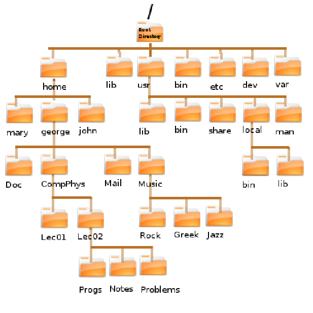
 user) obtains (
 others) and the group (
 group) loose (
 all) obtain read (
 (4th column =
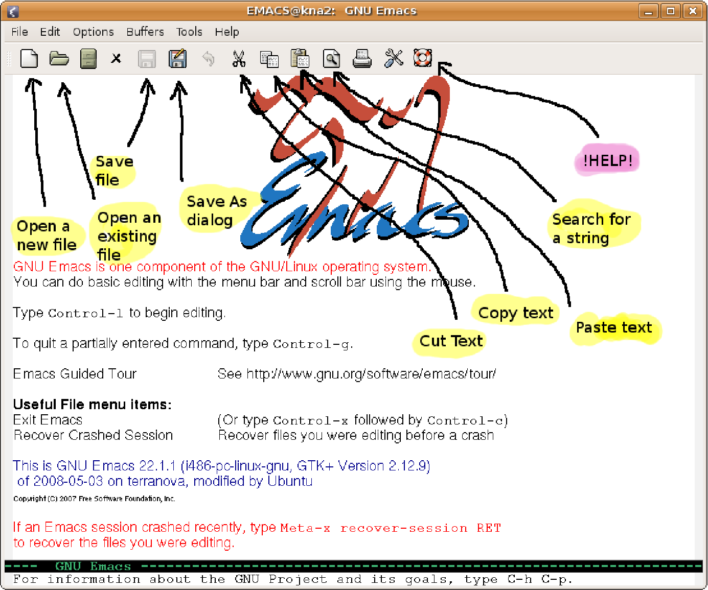
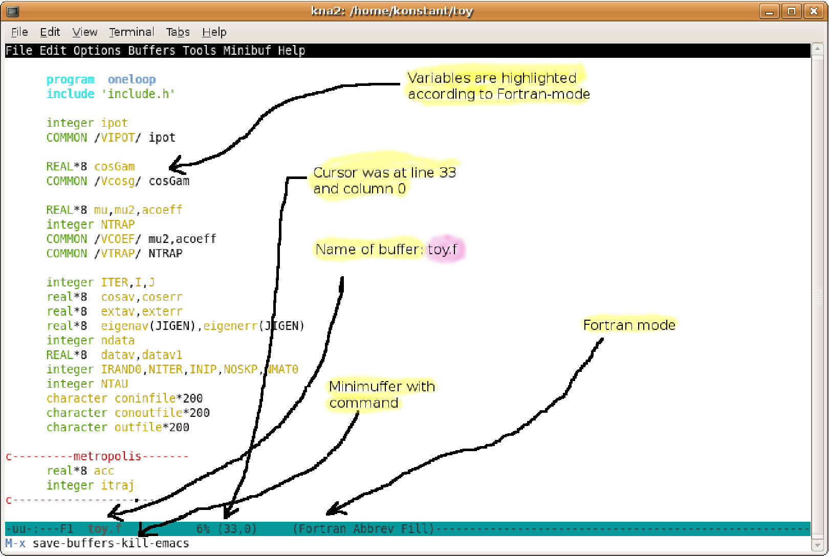
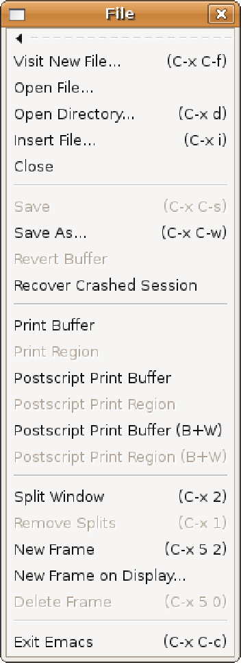

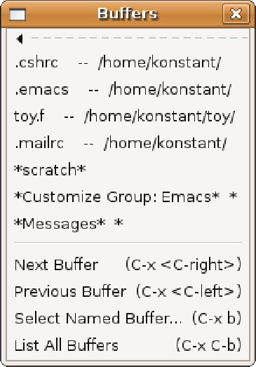
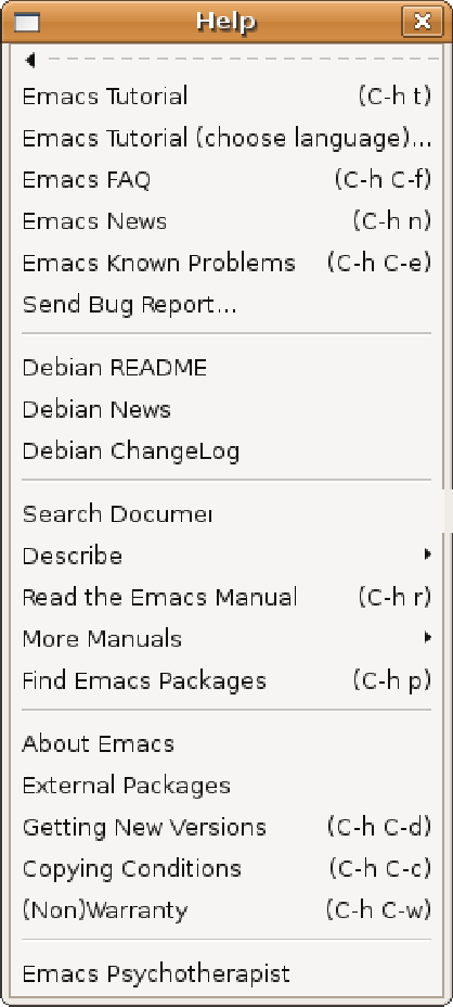


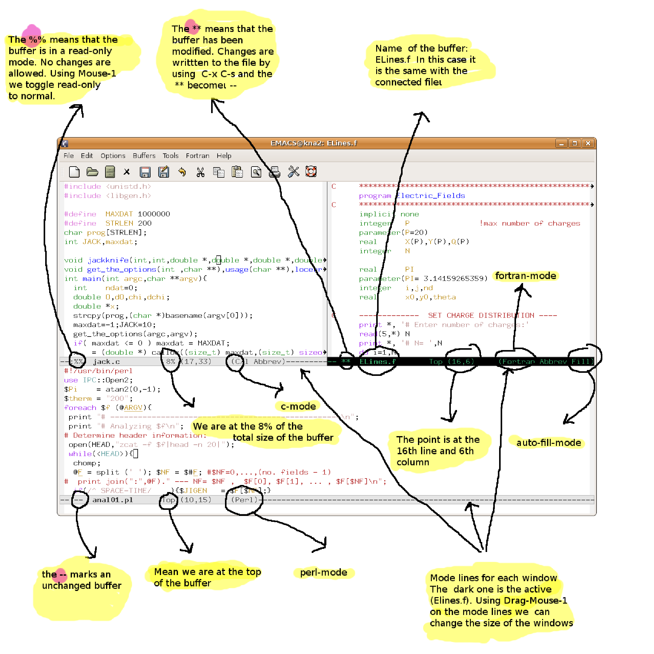


 and the area
  of the circle and printing the results. The
expressions
  ,
,  .
We will store the values of the radii in an
  . After a
check whether
  , it computes the discriminant
  by calling the
 which is a straight line with slope 1. In order to
plot many functions simultaneously, you can write all of them in one
line:
 ,
,  ,
,  and
and  .
Within the square brackets
  and
and  axes,
respectively. The bracket
  and the bracket
 . You may leave the job of setting such
limits to gnuplot, by omitting some, or all of them, from the respective
positions in the brackets. For example, typing
  and
and  and leaves the upper and lower limits
unchanged
 , we can read their values from files.
Assume that a file
  and
and  coordinates, respectively.
The keywords
  to the plot
with points.
 with a straight line
segment.
 . The second line
  .
.
 , where
  ,
,  and
and  are the numbers in the 2nd, 1st and
3rd columns respectively. The second line adds the plot of the function
 .
.
 .
After you make the plot, you can use the mouse in order to rotate it and view it
from a different perspective:
 and you want to create a plot of
 , write the data in a file, like in the following example:
 , where
  is a
parameter. A parametric plot in space (3-dimensions) is a surface

 , where
  are parameters. The following commands
plot the circle
  and the sphere

 :
: . These, as a function of time, describe the particle’s
trajectory. The position vector is
  , where
  and
and  are the
unit vectors on the
  and
and  axes respectively. The velocity vector is
 where
where 
 is given by
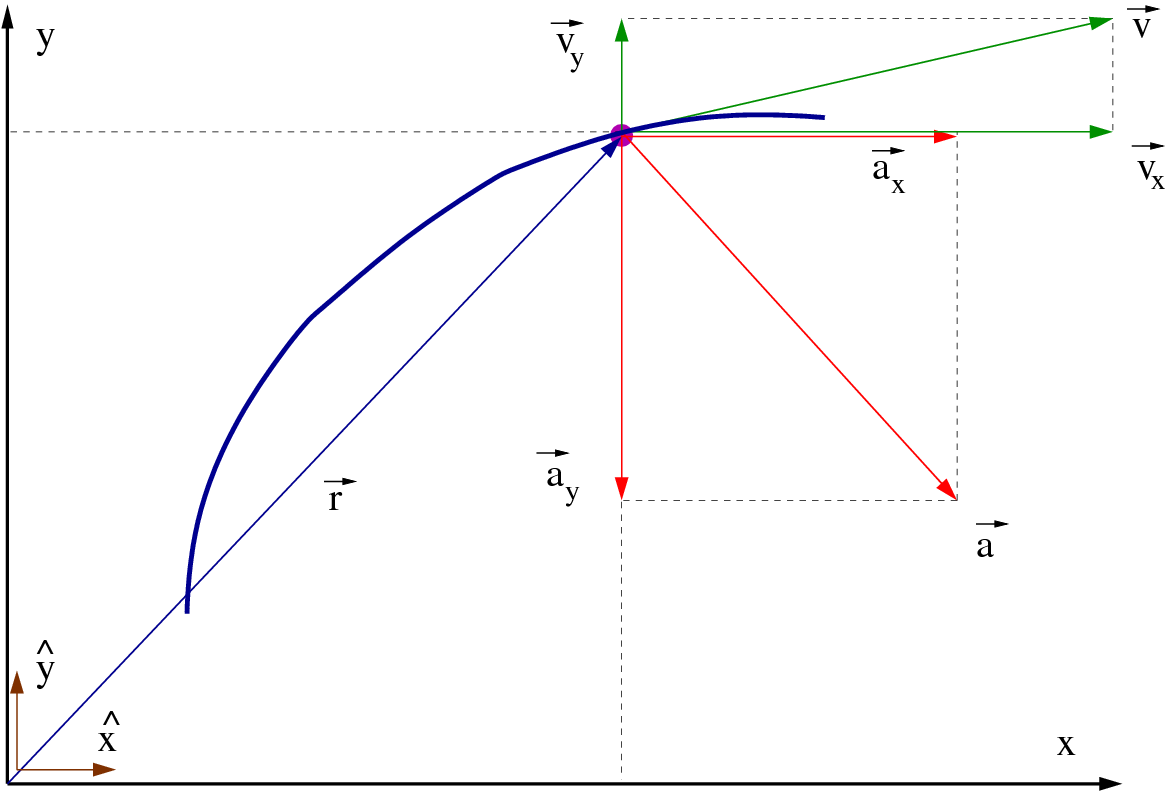


 are known. By taking their derivatives, we
can compute the velocity and the acceleration of the particle in motion. We will
write simple programs that compute the values of these functions in a time
interval
 ![[t0,tf]](main_latex88x.png) , where
, where  is the initial and
  is the final time. The continuous
functions
  are approximated by a discrete sequence
of their values at the times
  such that
 .
.
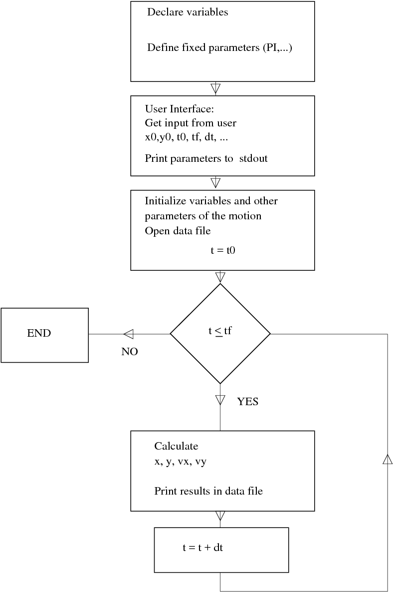
 ,
,  , etc). The program starts by interacting with
the user (“user interface”) and asks for the values of the variables
  ,
,
 ,
,  ,
,  ,
,  . The program prints these values to the
  . The values
of the positions and the velocities
  are calculated and
printed in a file together with the time
  . At this point we fix the format
of the program output, something that is very important to do it in a
consistent and convenient way for easing data analysis. We choose to
print the values t, x, y, vx, vy in five columns in each line of the output
file.
 and radius
  with constant angular velocity
  . The position on the
circle can be defined by the angle
  , as can be seen in figure
  to be
to be  .
.
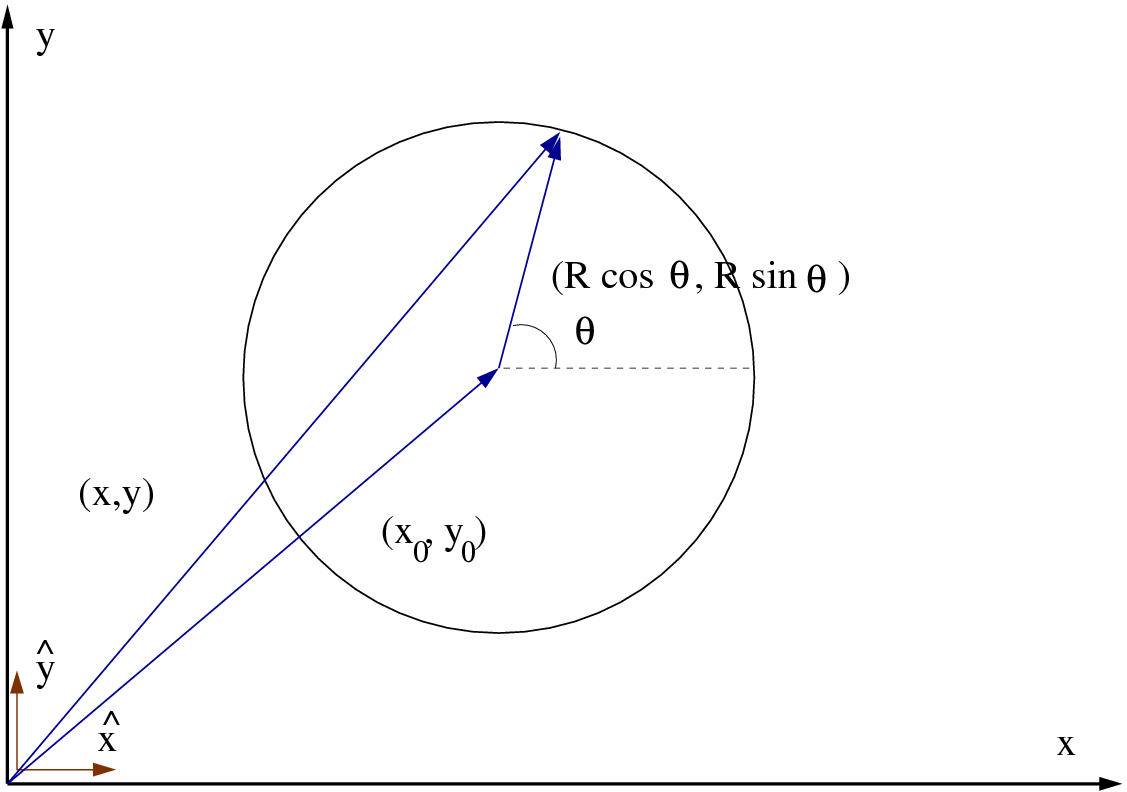
 are
are 
 we obtain the velocity

 (
( ,
,  ,
,
 tangent to the trajectory) and
  (
( and
and  anti-parallel,
 ).
).
 is stored
in the
  , the radius
  of
the circle and the angle
  are stored in the
  and are stored in the
  is calculated and stored in the
  in the
  and
and  . An
. An  or
or  the corresponding
  is also calculated and printed for reference.
 ,
,  ,
,
 ,
,  ,
,  and
and  .
.
 and
and  by using the
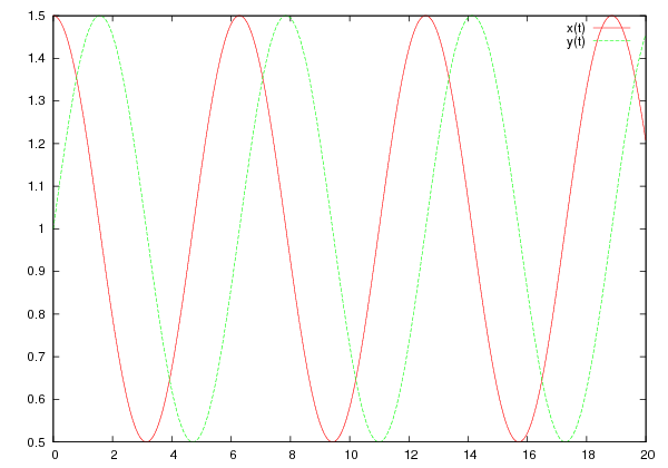


 . We can do that using
the raw data from the file
  . The function
  and
and  which mark the limit values of
  . The
. The  as function of time as well as the
trajectory
  can be plotted with the commands:
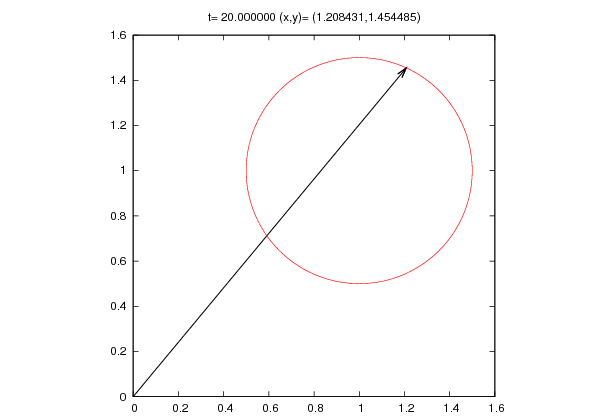
 , which
is the small angle that the pendulum forms with the vertical direction.


 and period
 . The angular velocity is computed from
  which gives

 and
and  . In order to
write the equations of motion in the Cartesian coordinate system shown in figure
2.6 we use the relations
 is hard coded in the program and
that the user can only set the length
  of the pendulum. The data file
 and the angular velocity
  .
.

 is the parameter. The initial conditions are
  ,
,
 and
and  , as shown in figure 2.7.
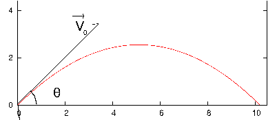


 in
in
 . The program calculates
  and
and  and prints them to the
  . The
solutions to the equations of motion
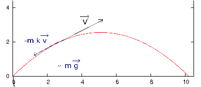


 ,
,  and
and  are
are
 . The full
program can be found in the file
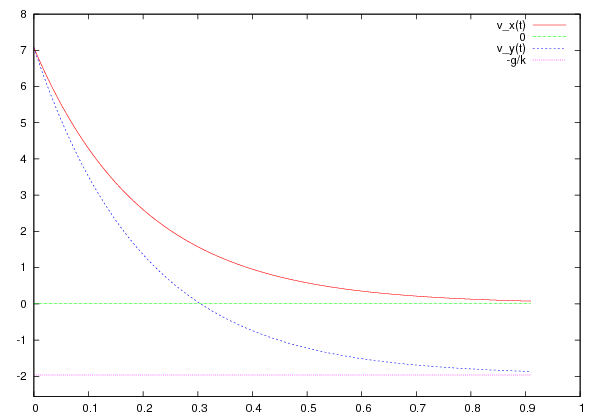


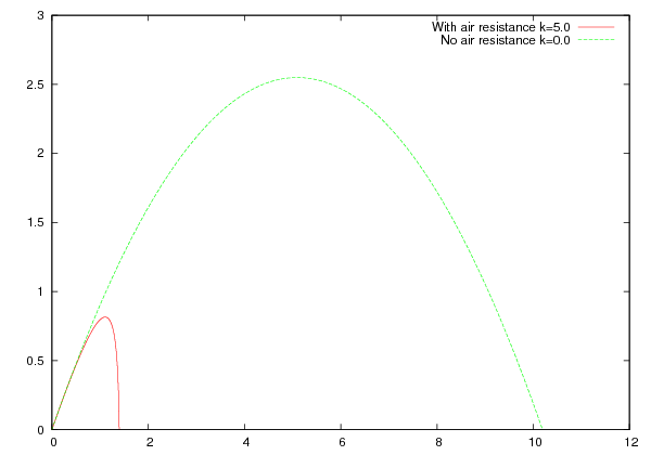


 and
and  are different in the
directions of the axes
  and
and  . The solutions of the dynamical equations
of motion for
  ,
,  ,
,  and
and  are
are

 and
and  satisfy certain relations, the trajectories of
the particle are closed and self intersect at a given number of points.
The proof of these relations, as well as their numerical confirmation, is
left as an exercise for the reader. The program listed below is in the file
 in the program above. The user must enter the two
angular frequencies
  and
and  and the corresponding times. A typical session
for the study of the problem is shown below:
 and
and  are shown in figure


 and the component of the
velocity
  . The structure of the programs will be exactly the same as
before.
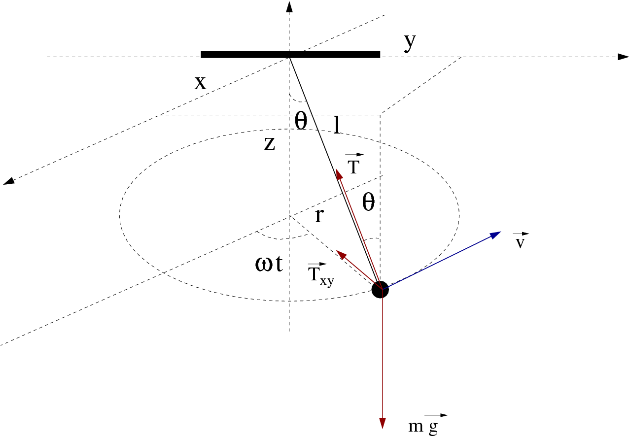
 plane with constant angular velocity
  . The
equations of motion are derived from the relations

 . Their solution


 ,
,  .
.
 ,
,  ,
the final time
  and the time step
  . We take
  . The convention that
we follow for the output of the results is that they should be written in a file
where the first 7 columns are the values of
  ,
,  ,
,  ,
,  ,
,  ,
,  and
and  . The
full program is listed below:
 ,
,  ,
,  ,
,  ,
,  ,
,  we give the following
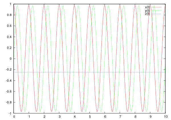
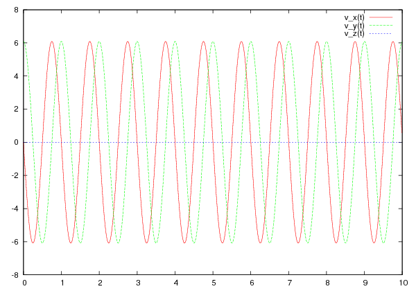


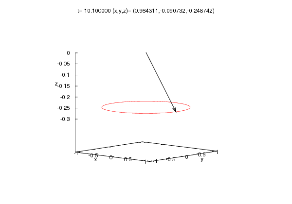


 . At time
  , the particle is at
  and its velocity
is
  , see figure
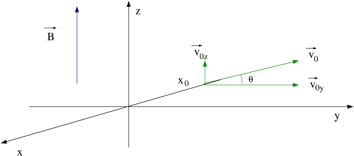


 and
the equations of motion are


 . This choice places the center of the circle,
which is the projection of the trajectory on the
  plane, to be at the origin of
the coordinate system. The trajectory is a helix with radius
  and pitch
 .
.
 and
and  , shown in figure
  (Larmor frequency). The components of the initial
velocity are
  and
and  . The initial position is calculated
from the equation
  . The program can be found in the file
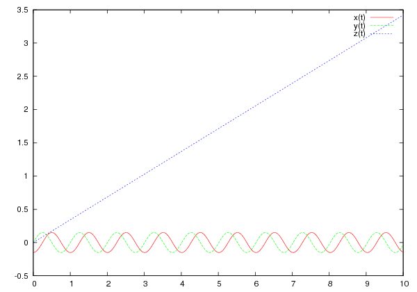
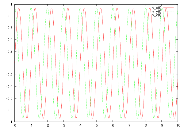


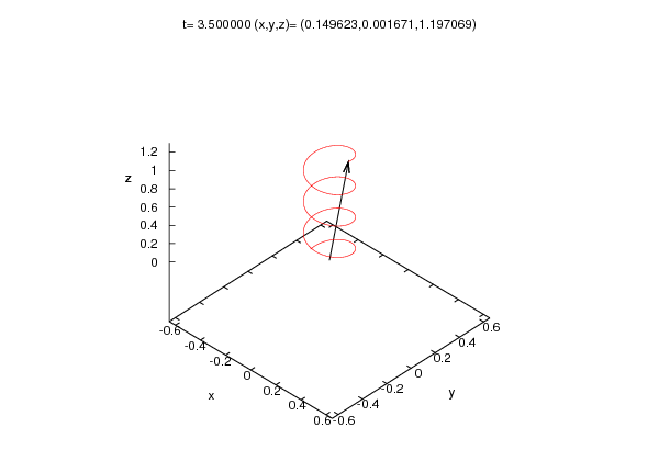


 axis for
  , as
can be seen in figure
  and
and
 it bounces and its velocity instantly reversed. Its potential energy
is

 within the box and
  at the position of the walls.


 as well as its velocity
 (the sign of
  depends on the direction of the particle’s motion) at time
 . As long as the particle moves within the box, its motion is free and

 , so that there is no bouncing on the wall in
the time interval
  , we have that
 . The devil is
hiding in the word “when”. Since the time interval
  is finite in our program,
there is no way to know the instant of the collision with accuracy better than
 . However, our algorithm will change the direction of the velocity
at time
  , when the particle will have already crossed the wall.
This will introduce a systematic error, which is expected to decrease with
decreasing
  . One way to implement the above idea is by constructing the
loop
 while
while  . Note that variables of the integer type (
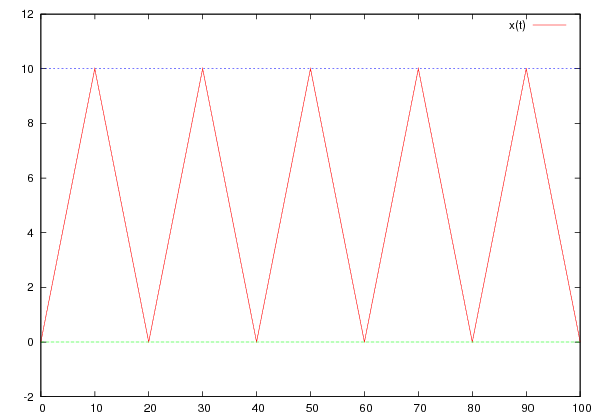
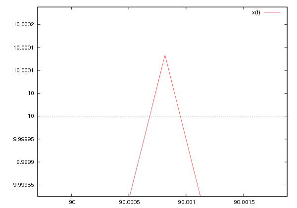


 is shown in figure
  units of time. Therefore, on the plot to the right of figure
  ,
,
 .
.
 . Therefore, we naively expect that
as long as we have the necessary computer power to take
  as small as possible
and the corresponding time intervals as many as possible, we can achieve any
precision that we want. Well, that is true only up to a point. The problem is that
the next position is determined by the addition operation

 , but some degree
of accuracy is also lost at each addition operation. And since we have
accumulation of such errors over many intervals

 limit
limit .
Then, the systematic error that accumulates with each addition of two numbers
with increasing difference in their orders of magnitude. This error is
  . The competition of the two effects makes the optimal choice
of
  the result of a careful analysis. Such a situation is found in many
interesting problems, therefore it is quite instructive to study it in more
detail.
 . If the
solutions are converging in a region of values of
  , one gains confidence
that the true solution has been determined up to the accuracy of the
convergence.
 by fixing all the parameters except
  and then study
the dependence of the results on
  . We will take
  ,
,  ,
,
 ,
,  ,
,  , so that the particle will collide with the
wall every 10 units of time. We will measure the position of the particle

 and study its convergence to a
limit
 .
.
 for
many values of
  . We write the values of the parameters read by the program in
a file
  can be found
in the last line of the file
  and the first two numbers coming out from
the command
  in the file
 reaches the
value
 .
We do the same
 in two new columns in the
file
  , whereas for
  the error becomes
  % and the
method becomes useless. The 2nd method has much better behavior that the 1st
one.
 decreases, the final value of
  approaches the
expected
  . Why don’t we obtain
  , especially when
  is an
integer? How many steps does it really take to reach
  , when the expected
number of those is
  ? Each time you take a measurement, issue the
command
 and in the end the difference is about 5%! Notice
that the last line should have given
  , an error
comparable to the period of the particle’s motion.
 . We can improve the accuracy of the calculation significantly if we
use the multiplication
  does not
vanish completely due to the operation
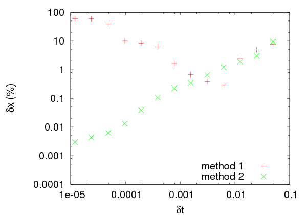
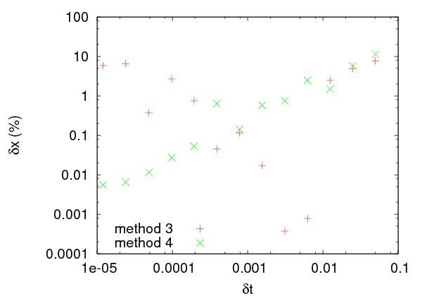


 and
and
 . When it reaches the boundaries of this two dimensional box, it
bounces elastically off its walls. The particle is found in an infinite depth
orthogonal potential well. The particle starts moving at time
  from
from  and our program will calculate its trajectory until time
  with time step
  .
Such a trajectory can be seen in figure
  , then at time
 they will be given by the relations

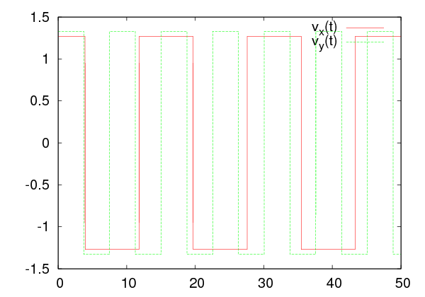


 and
and
 and which is open on the
  side. In the box there is a circular “hole”
with center at
  and radius
  . If the “ball” falls in the “hole”, the player
wins. If the ball leaves out of the box through its open side, the player
loses. In order to check if the ball is in the hole when it is at position
 , all we have to do is to check whether
  .
.
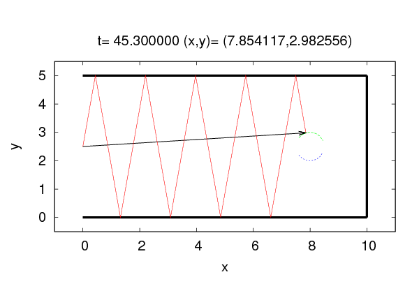


 at time
  . The
player hits the ball which leaves with initial velocity of magnitude
  at an angle
 degrees with the
  axis. The program is found in the file
  and height
  . The collisions of
the particle with the cylinder are elastic. We take the axis of the cylinder to be
the
  axis and the two bases of the cylinder to be located at
  and
and  .
This is shown in figure
  plane. The projection of the particle moves within a circle of radius
  and center at the intersection of the
  axis with the plane. This is shown in
figure
  component of the velocity is reflected
 , whereas
  remains the same. The velocity of the particle before the
collision is


 ,
,  , we have that

 , the new velocity in Cartesian coordinates
will be
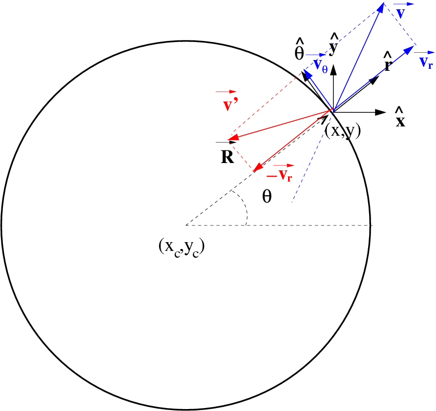


 ,
,  will be performed in the
function
  .
.
 in radians. The correct quadrant of the circle where
  lies
is chosen. The angle that we want to compute is given by
  , exactly on the circle.
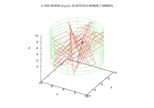


 as a function of time using the command:
 . The cylinder (without the
bases) is given by the parametric equations
  with
with  ,
, ![v ∈ [0,L ]](main_latex471x.png) .
.

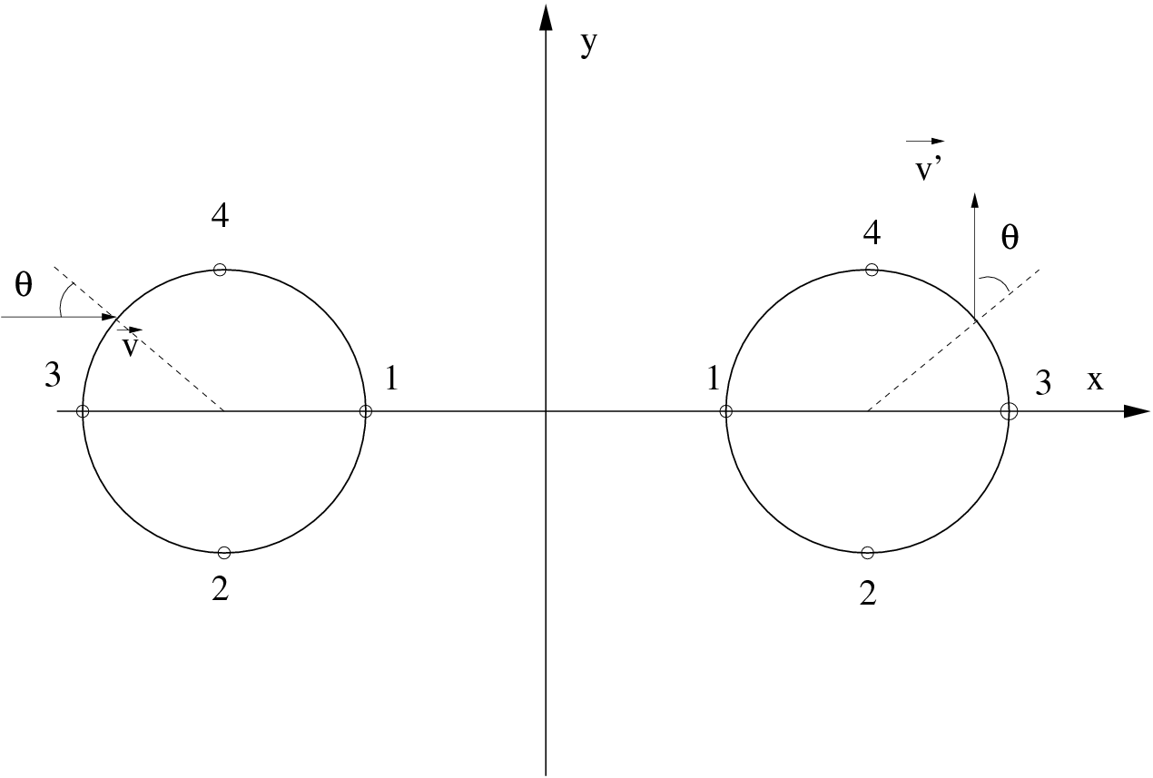


 with
centers at distance
  like in figure
  ,
,  ,
,
 for the right circle and
  ,
,  ,
,
 for the left. Points on the two circles with the same
  are
identified. A particle entering the wormhole from the left circle with velocity
  is
immediately exiting from the right with velocity
  as shown in figure
 and
and  . We will use periodic
boundary conditions in order to define what happens when the
particle attempts to move outside these limits. This means that we
identify the
  line with the
  line as well as
the
  line with the
  line. The user enters the
parameters
  ,
,  and
and  as well as the initial conditions
  ,
,
 where
where  . The user will also provide
the time parameters
  and
and  for motion in the time interval
![t ∈ [t = 0,t ]
0 f](main_latex503x.png) with step
with step  .
.
 ,
, 
 ,
,  in
the geometry with
  .
.
 ,
,  and determine whether it is stable under small
perturbations of the initial conditions.
 and moves in
the
  direction to the
  ,
,  position, draw the
trajectory and calculate the distance traveled on paper. Then confirm
your calculation from the numerical result coming from your program.
 ,
,  and replot all the trajectories
mentioned above.
 by the parametric equations

 by the parametric equations

 by
by 
 for given
  ,
,  and as long as
  . If the point
 is outside the boundaries
  ,
,  , we redefine
 ,
,  in each case respectively. Points defined by the same
value of
  are identified, i.e. they represent the
  crosses either one of the circles
  or
or  , then we take the particle out
from the other circle.
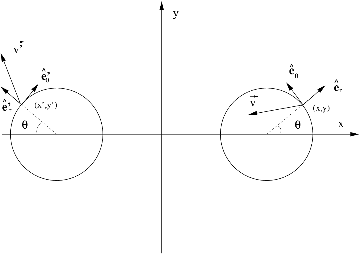


 is determined by the relation

 is calculated from the equation

 is mapped to the point
  where
where

 , we first calculate the
vectors


 and
and  . Therefore, the
relations that give the “emerging” velocity
  are:
are:

 and emerging from
  .
The condition now is:

 is given by

 is mapped to the point
  where
where

 , we calculate the vectors


 is:
is:

 ,
,  (why?). Try to think of ways to control those errors and
study them.

 .
.

 and
and  respectively. They are also
unstable, as can be easily verified by using the program that you will write. The
full program is listed below:
 on a circle that
has the origin of the coordinate system at its center. At time
  ,
the particle is at
  . Write the program
  . The program should print the results
like the program
  limit in the projectile motion given by equations
(
 and keep the non
vanishing terms as
  . Then keep the next order leading terms
which have a smaller power of
  . Program these relations in a file
 and calculate the range of the trajectory numerically by
using the two programs
  for which the two results agree within 5% accuracy.
 . Repeat by taking the amplitude in the
 direction to be twice as much the amplitude in the
  direction.
 case.
case.
 plane makes during its motion.
 ,
,  with the walls.
 ,
,  ,
,
 .
.
 . Upon reaching the ground, it bounces
inelastically such that
  with
with  a parameter. Write
the necessary program in order to study numerically the particle’s
motion and study the cases
  .
.
 . Animate the calculated trajectories.
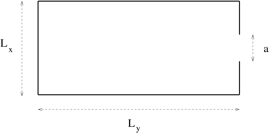


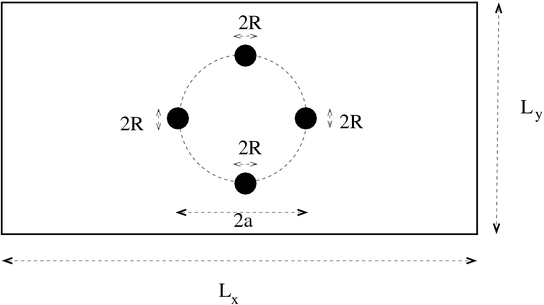
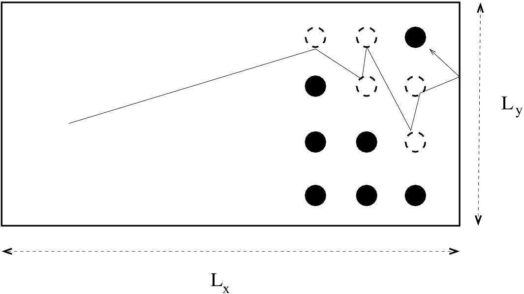
 of a population
  is
proportional to the current population:

 showing an
 an decline for
  . It is obvious that
this model is reasonable as long as the population is small enough so that the
interaction with its environment (adequate food, diseases, predators etc)
can be neglected. The simplest model that takes into account some of
the factors of the interaction with the environment (e.g. starvation) is
obtained by the introduction of a simple non linear term in the equation so
that

 gives the maximum growth rate of the population and
  controls the ability of the species to maintain a certain population level. The
equation (
 and that the n-th generation has population
  where
where  . Then
  and equation (
 . The solutions of the above equation are well approximated
by
 so that we have population growth when
 and decline when
  . Equation (
 we obtain the logistic map

 is considered as a given
parameter), so that

 ,
,  ,
,  ,
,
 for function composition. In what follows, the derivative of
  will be
useful:

 to be the fraction of the population with
respect to its maximum value, we should have
  for
each
 . The function
  has one global maximum for
  which is equal
to
  . Therefore, if
  , then
  , which for an
appropriate choice of
  will lead to
  for some value of
  .
Therefore, the interval of values of
  which is of interest for our model
is

 , a sequence
of values


 is produced. This will be
referred
 . In the following sections we will study the properties of
these trajectories as a function of the parameter
  .
.
 we have


 ,
,  whereas for
  we have periodic trajectories
resulting in rational
  and non periodic resulting in irrational
  . For other
values of
  we have to resort to a numerical computation of the trajectories of
the logistic map.
 Cycles
 is a solution of the equation
  , then


 for every
  . For the function
  we have two solutions
 , these solutions are
  , the sequence
  approaches asymptotically one of these points as
 . Obviously the (measure zero) sets of initial values
  and
and
 result in trajectories attracted by
  and
and  respectively. In
order to determine which one of the two values is preferred, we need to study the
 and
and  . For this, assume that for some
value of
 ,
,  is infinitesimally close to the fixed point
  so that


 about
about
 and the relation
  , we have that
  . Then we
obtain

 we obtain
  and the fixed point
  is
is
 approaches
  asymptotically. If
  then the sequence
  deviates away from
  and the fixed point is
 should be studied separately
and it indicates a change in the stability properties of the fixed point. In
the following discussion, these points will be shown to be bifurcation
points.
 with
with  we have that
 and
and  . Therefore, if
  the point
  is an
attractor, whereas the point
  is irrelevant. When
  ,
the point
  results in
  , therefore
  is unstable.
Any initial value
  near
near  deviates from it. Since for
  we
have that
  , the point
  is an attractor. Any
initial value
  approaches
  . When
  we
have the limiting case
  and we say that at the critical value
 the fixed point
 and
and
 .
.
 increases, the fixed points continue to bifurcate. Indeed, when
 we have that
  and for
  the point
  becomes unstable. Consider the solution of the equation
  . If
. If
 is one of its solutions and for some
  we have that
  , then


 and
and 


 (therefore
  is also a solution). If
 are two such
  ,
,  , then the
trajectory is periodic with period 2. The points
  ,
,  are such that they are


 of the
equation
 , the polynomial above can be written in the form (see
 ,
,  and
and  . The
roots of the trinomial in (
 . For the values of
  of interest (
 ), the
discriminant becomes positive when
  and we have two different
solutions

 we have one double root, therefore a unique fixed point.
 requires
the same steps that led to the equation (
 is greater, less or equal to one. By noting
that


 , we see that for
 ,
, 
 and for
  ,
,

 . For the intermediate values
  the
derivatives
  for
for  . Therefore, these points are stable
solutions of
  and the points
  bifurcate to
  ,
,  for
for  . Almost all trajectories with initial points in the interval
![[0,1]](main_latex814x.png) are attracted by the periodic trajectory with period 2, the “2-cycle”
are attracted by the periodic trajectory with period 2, the “2-cycle”
 .
.
 ,
,  bifurcate to the eight fixed points
  ,
,  when
when  .
These are real solutions of the equation that gives the 4-cycle
  .
For
.
For  , the points
  ,
,  are a stable
4-cycle which is an attractor of almost all trajectories of the logistic
map
 the 16 fixed points of the equation
 give a stable 8-cycle, for
  a stable 16-cycle
etc
 are getting closer to each other as
  increases so that
 . As we will see,
  marks the onset
of the non-periodic, chaotic behavior of the trajectories of the logistic
map.
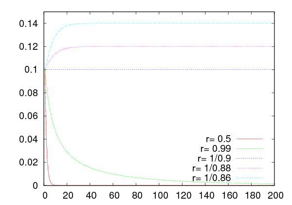
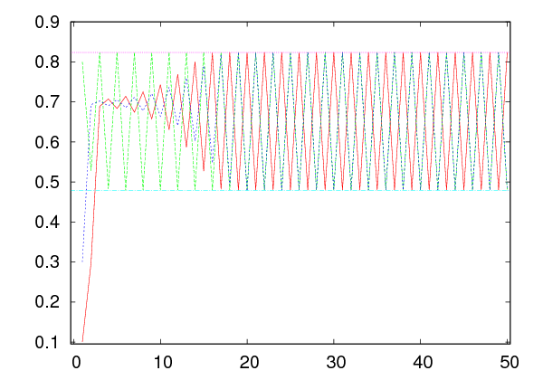


 and
and
 . The program can be found in the file
  goes past the values
  and
and  . Similarly, we can study
trajectories which are
  -cycles when
  crosses the values
  .
.
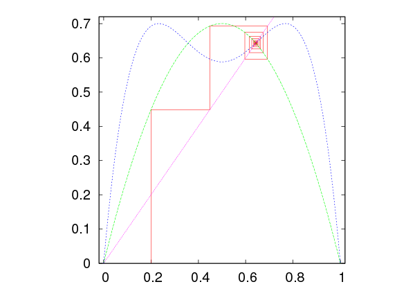


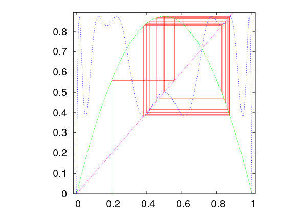


 and we calculate the point
  , where
 . This point belongs on the curve
  . The point
  is
then projected on the diagonal
  and we obtain the point
  . We
repeat
  times obtaining the points
  and
and  on
on  and
and  respectively. The fixed points
  are at the intersections of
these curves and, if they are attractors, the trajectories will converge on them. If
we have a
  -cycle, we will observe a periodic trajectory going through
points which are solutions to the equation
  . This exercise can
be done by using the following program, which can be found in the file
 ,
,  and of the diagonal
 . Figures
  .
.

 ,
,  ,
,  and
and 
 .
For
.
For  we have
  fixed points
  ,
,  of
of
 . By plotting these points
  as a function of
  we construct
the bifurcation diagram. These can be calculated numerically by using the
program
  that
she needs to study and for each one of them the program records the point of the
 -cycles
 ,
,  . This is easily done by computing the
logistic map several times until we are sure that the trajectories reach the stable
state. The parameter
  -cycles or depict a dense
enough set of values of the non periodic orbits. The program is listed
below:
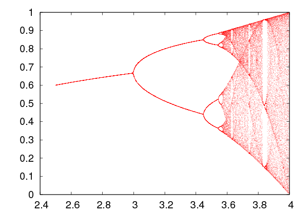
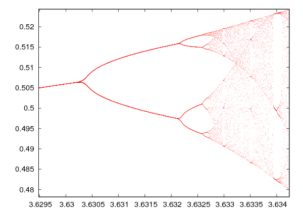


 -cycles for
  . When
  goes
past
  , the trajectories become non-periodic and exhibit chaotic behavior.
Chaotic behavior will be discussed more extensively in the next section. For the
time being, we note that if we measure the distance between the points
 , we find that it decreases constantly with
  so
that

 is the Feigenbaum constant
 , defined by the
quotient of the separation of adjacent elements
  of period doubled attractors
from one double to the next
  , is
, is

 ! By using the theorem of Sharkovskii, Li and
Yorke
 in exactly the same way that we did in
equations (
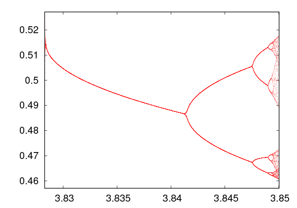

 ,
,  and
and  .
The constants
  and
and  of equations (
 and
and  . For
this reason, one has to use an approximate numerical calculation of the
roots, and the simple Newton-Raphson method will prove to be a good
choice.
 for the solution of the
equation
  and computes a sequence of points


 that presumably converges to one of the roots of the equation.
The computation stops at a finite
  , when we decide that the desired
level of accuracy has been achieved. In order to understand how it works,
we assume that
  is an analytic function for all the values of
  used in the computation. Then, by Taylor expanding around
  we
obtain

 , we choose

 of one variable
  . Different choices for
  will possibly lead to
different roots. When
  ,
,  are non zero at the root and
  is
bounded, the convergence of the method is quadratic with the number of
iterations. This means that there is a neighborhood of the root
  such that the
distance
  is
is  . If the root
  has multiplicity
larger than 1, convergence is slower. The proofs of these statements are simple and
can be found in
  for some
  , the method
stops. For functions that tend to
  as
as  , it is easy to make a bad choice
for
  that does not lead to convergence to a root. Sometimes it is a
good idea to combine the Newton-Raphson method with the
  diverges at the root we might get into
trouble. For example, the equation
  with
with  , does
not lead to a convergent sequence. In some cases, we might enter into
non-convergent cycles
  that will converge to the root) can be tiny. See problem

 in a one dimensional potential well
of depth
  and width
  . The parameters
  and
and
 . Given
  , we solve for
  which gives the energy
  . The
function
  and its derivative
  are
are 
 can be found in the file
  . We
fix
 . It is instructive to make the plot of the left and right hand
sides of (
 .
Using
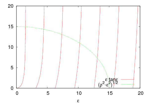

 .
The reader can compute more of these roots by following these steps by
herself.
 and
and  . In order to compute a sequence
  ,
,
 ,
,  ,
,  ,
,  ,
,  that may converge to a root
of the above system of equations, we Taylor expand the two functions around

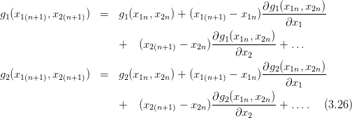
 and
and  and setting
 ,
,  , we obtain
 system of equations
 and
and  , with
  . Solving for
  we obtain

 become small enough.
 ,
,
 . We have
  ,
,  ,
,  ,
,
 . The program can be found in the file
  together with the plane
  . The intersection
of the three surfaces determine the roots we are looking for. Compiling and
running the program can be done by using the commands:

 ,
,

 ,
, 
 .
.
 we will solve the algebraic
equations
  and
and  . At these points,
  -cycles
become unstable and
  -cycles appear and are stable. This happens when
 , where
  . We will look for solutions
  for
for
 .
.
 and
and  as in equation (
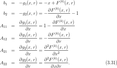


 by a routine that will compose the function
 -times. The
program can be found in the file
  with the expected one
 . Improving the accuracy
of the calculation is left as an exercise for the reader who has to control the
systematic errors of the calculations and achieve better accuracy in the
computation of
  .
.
 , the trajectories of the logistic map
become non periodic and exhibit chaotic behavior. Chaotic behavior mostly
means sensitivity of the evolution of a dynamical system to the choice of initial
conditions. More precisely, it means that two different trajectories constructed
from infinitesimally close initial conditions, diverge very fast from each other. This
implies that there is a set of initial conditions that densely cover subintervals of
 whose trajectories do not approach arbitrarily close to any cycle of finite
length.
 ,
,  as initial points and
 . When the points
  ,
,  have a distance
  that for small enough
  increases exponentially with
  (the “time”),
i.e.

 is called a
  is
is

 so that
 . Then we obtain
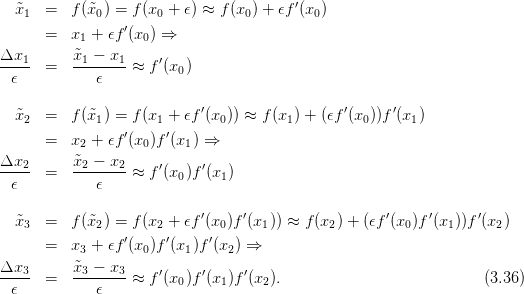
 and by
taking the logarithm and the limits we can prove (3.35) .
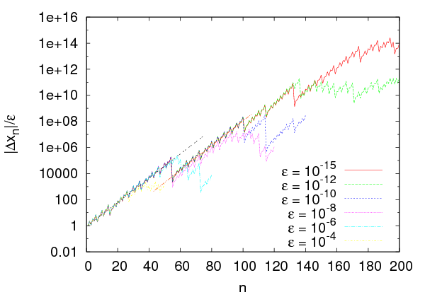


 is found at the fourth column
of the file
  ,
,  ,
,  and
and
 . The
. The  tend to lie on a straight line as
  decreases. The slopes of these lines are
equal to the Liapunov exponent
  . Deviations from the straight line
behavior indicates corrections and systematic errors, as we point out in figure
 , and the true value can be estimated as the average over several such
choices. We estimate the error of our computation from the standard
error of the mean. The reader should perform such a computation as an
exercise.
 to the exponential function in
the following way: Since
 , we can
make a fit to a straight line instead. Using
  (
(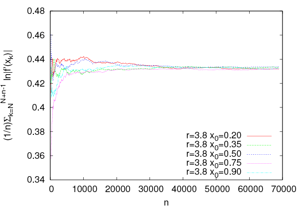


 . This equation is
approximately correct when (a) we have already reached the steady state and (b)
in the large
  limit. For this reason we should study if we obtain a satisfactory
convergence when we (a) “throw away” a number of
  (c) calculate the sum (
 . This has to be carefully repeated
for all values of
  since each factor will contribute differently to the
quality of the convergence: In regions that manifest chaotic behavior (large
 ) convergence will be slower. The program can be found in the file
 . At each step the sum divided by the number
of steps
  . This is a point where the system exhibits strong chaotic
behavior and convergence is achieved after we compute a large number
of steps. Using
  and
and  the achieved
accuracy is about
  % with
  . The
main contribution to the error comes from the different paths followed by
each initial point chosen. The plot can be constructed with the
  ,
,
 ,
,  and
and  and plots the
results from the contents of the file
  on the value of
  . Using our experience
coming from the careful computation of
  before, we will run the program for
several values of
  using the parameters
  ,
,  from the initial point
  . This calculation gives accuracy of the order of
 %. If we wish to measure
  carefully and estimate the error of the results, we
have to follow the steps described in figures
  .
.
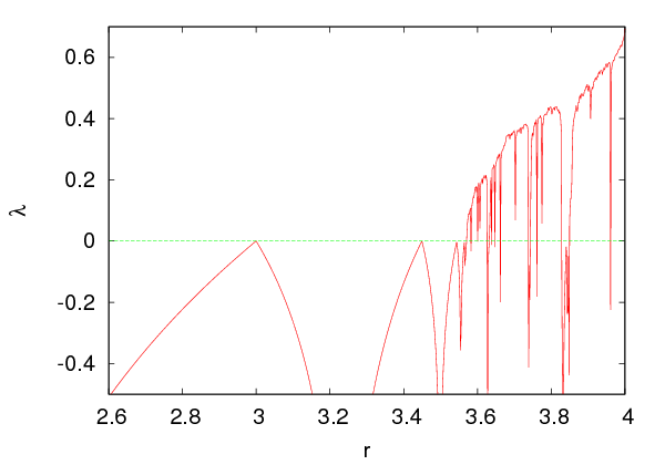


 correspond to stable
  -cycles. The intervals where
 correspond to manifestation of
  where the system exhibits
  instead of an exponential, where
  is
a positive exponent that needs to be determined. The parameter
  is
the one usually used in the literature. Strong chaos is obtained in the
 limit. For larger
  , switching between chaotic and stable periodic
trajectories is observed each time
  changes sign. The critical values
of
  can be computed with relatively high accuracy by restricting the
calculation to a small enough neighborhood of the critical point. You can do
this using the program listed above by setting the parameters
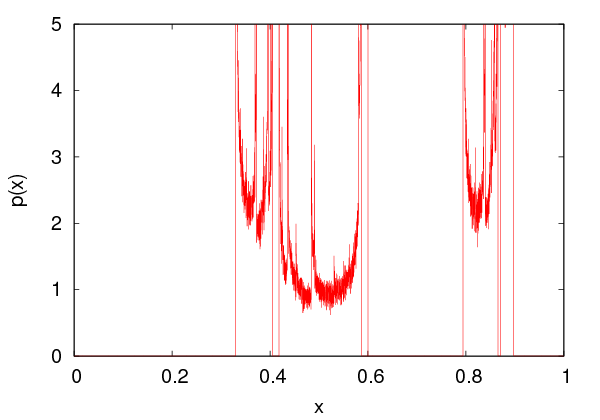
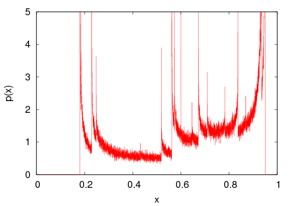


 of the values of
  in the interval
  .
After the transitional period, the distribution
  for the
  cycles will have
support only at the points of the
  cycles, whereas for the chaotic regimes it will
have support on subintervals of
  . The distribution function
  is
independent for most of the initial points of the trajectories. If one obtains a large
number of points from many trajectories of the logistic map, it will be
practically impossible to understand that these are produced by a deterministic
rule. For this reason, chaotic systems can be used for the production of

 is the probability of observing the state
  . In our case, we can make
an approximate calculation of
  by dividing the interval
  to
to  subintervals of width
  . For given
  we obtain a large number
  of values
 of the logistic map and we compute the histogram
  of their distribution in
the intervals
  . The probability density is obtained from the limit
of
  as
as  becomes large and
  small (large
  ).
Indeed,
  converges to
  . We will define
 .
.
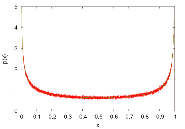


 for chosen values of
  , and then the
entropy
  is calculated using (
 for the histograms. The probability density is
calculated in the array


 and the width
  ,
so it should be large enough. The parameter
  and it should be large enough in
order to reduce the “noise” in
  . It is obvious that
  becomes smaller. Appropriate choices lead to the plots
shown in figures
  ,
,  and
and  . We see that
stronger chaotic behavior means a wider distribution of the values of
 .
.
 , which
increases even further as the chaotic behavior becomes stronger. During the
intermissions of the chaotic behavior there are sudden drops in the value of the
entropy. It is quite instructive to compare the entropy diagrams with the
corresponding bifurcation diagrams (see figure
  reaches its maximum value 4, but this is not done smoothly. By magnifying
the corresponding areas in the plot, we can see an infinite number of
sudden drops in the entropy in intervals of
  that become more and more
narrow.
 are falling off
exponentially for large enough
  .
.
 and plot the trajectories for
  with
step
  for
for  . Put the
  axis in a logarithmic
scale. From the resulting curves discuss whether you obtain an
exponential falloff.
 for
for  to the function
  and determine
the fitting parameters
  and
and  . How do these parameters depend on
the initial point
  ? You can use the following
  , therefore avoiding the transitional
period and the deviation from the exponential falloff for small
 .
.
 with step
  and for
  . As
you will be approaching
  , you will need to discard more
points from near the origin. You might also need to increase
 for large
 . Construct a table for the values of
  as a function of
 .
. . How is this related to the
values that you computed in your table?
 . Choose
  and compare
your result to the known value
  . Repeat for
  for
for
 . What do you conclude about the point
 ?
?
 . Calculate the stable
point
  and compare your result to the known value
  .
How large should
  . Take
  and
and  by using the command
  . How big should
  and
and  with an accuracy of 6 significant
digits?
 and
and  . Choose
  -
- and
and
 -
- .
.
 ,
,  ,
,  ,
,  for given
  on the same
graph. Use the commands:
 . Take
  ,
,  ,
,  ,
,  ,
,
 . Determine the fixed points and the
  -cycles from the intersections of
the plots with the diagonal
  .
.
 and
and  .
Repeat by dropping from the plot an increasing number of initial points, so
that in the end only the
  -cycles will remain. Do the same for
 .
.
 and for
  . Compute the first four bifurcation points with
an accuracy of 5 significant digits by magnifying the appropriate parts of the
plots. Take
  .
Compute graphically the bifurcation points
  for
for 


 . Make sure that your results are stable against variations of the
parameters
  for
for  , and from the
dependence of your results on the choices of
  and compare your results to equation (
 in equation (
 . Find the
roots obtained by the Newton-Raphson method when you choose


 .
What do you conclude concerning the basins of attraction of each root of the
polynomial? Make a plot of the polynomial in a neighborhood of its roots
and try other initial points that will converge to each one of the roots.
 of the logistic map. Use appropriate areas of the bifurcation
diagram so that you can choose the initial points correctly. Check that
your result for
  is the same for all
  . Tune the parameters
chosen in your calculation on order to improve the accuracy of your
measurements.
 and
and  .
.
 and
and  .
.
 for
for  of the logistic map
using the Newton-Raphson method. In order to achieve that, you should
determine the bifurcation points graphically in the bifurcation diagram first
and then choose the initial points in the Newton-Raphson method
appropriately. The program in
  . If these parameters are too small the
convergence will be unstable and if they are too large you will have large
systematic errors. Using this method, try to reproduce table


 of equation (
 and the critical value
  by
assuming that for large enough
  ,
,  . This behavior
is a result of equation (
 and
and  . This hypothesis is confirmed in
figure
  to
to  . Construct the same plot using the parameters of your
calculation.
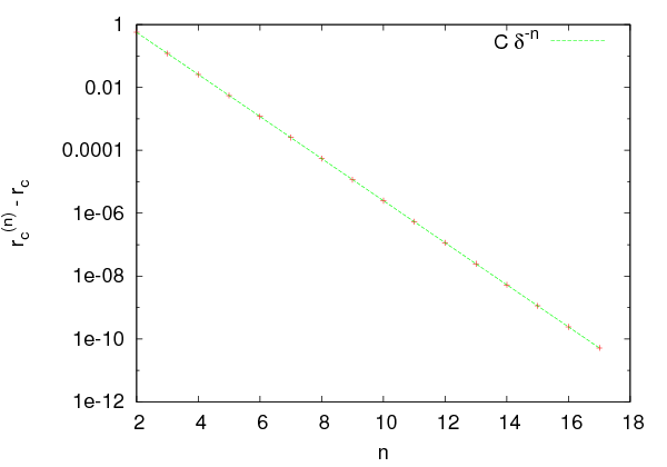


 . Choose one
bifurcation point of the 3-cycle, one of the 6-cycle and one of the 12-cycle
and magnify the bifurcation diagram in their neighborhood.

 ,
,  ,
,  ,
,  for
for  ,
,
 ,
,  ,
,  for
for  . For which values of
  do you
expect to obtain stable
  -cycles?
 plot the trajectories with initial points
 . For each
  make a separate plot.
 for
for  as well as the first two bifurcation points of
the 3-cycle.
 . Determine
the point marking the onset of chaos as well as the point where
the 3-cycle starts. Magnify the diagram around a branch that you
will choose.
 as in problem
  ? Is the value of
  the same as that of the logistic map?
 ,
,  ,
,  ,
,  ,
,  for
for
 ,
,  ,
,  ,
,  ,
,  . Which values of
  are
expected to lead to stable
  -cycles?
 , plot the trajectories with initial points
 . Make one plot for each
  .
.
 for
for  as well as the first two bifurcation points of
the 3-cycle.
 . Within which
limits do the values of
  lie in? Repeat for
  . What
do you observe? Determine the point marking the onset of chaos
as well as the point where the 3-cycle starts. Magnify the diagram
around a branch that you will choose.
 . Within which
limits do the values of
  lie in? Determine the point marking
the onset of chaos as well as the point where the 3-cycle starts.
Magnify the diagram around a branch that you will choose.
 for
for  as well as the first two bifurcation points of
the 3-cycle.
 . Within which limits do
the values of
  lie in? On the same graph, plot the functions
  ,
,
 .
.
 and
and  .
At which point do the two disconnected intervals within which
  take their values merge into one? Magnify the areas
  ,
,
 and
and  ,
,  and determine the merging points of two disconnected intervals within
which
  take their values.

 and
and 

 . Make your program to take as the initial point of the new
trajectory to be the last one of the previous trajectory and choose
 for
for  . Repeat for
  . What do you
observe? Note that as
  is increased, we obtain bifurcations and
“anti-bifurcations”.
![xn+1 = [xn + r − q sin(2πxn )] mod1.](main_latex1400x.png)
 so that
  ).
Construct the bifurcation diagram for
  and
and  .
.
 that originally are at a
distance
  . Choose


 and calculate the Liapunov exponent by fitting
to a straight line appropriately. Compute the mean value and the standard
error of the mean.


 for the logistic map. Use both ways mentioned in the text. Choose at least 5
different initial points and calculate the mean and the standard error of the
mean of your results. Compare the values of
  that you obtain with each
method and comment.
 numerically as the limit
  for the
logistic map with an accuracy of nine significant digits. Use the
calculation of the Liapunov exponent
  given by equation (
 of the logistic map numerically for which
we (a) enter a stable 3-cycle (b) reenter into the chaotic behavior.
Do the calculation by computing the Liapunov exponent
  and
compare your results with the ones obtained from the bifurcation
diagram.
![r(1−xn)
xn+1 = xne , 1.8 < r < 4
xn+1 = r sin (πxn), 0.6 < r < 1
2
xn+1 = 1 − rx n, 0 < r < 2
xn+1 = e− rx2n + q, r = 7.5,− 1 < q < 1
[ ]
xn+1 = xn + 1-− q sin(2πxn ) mod1, 0 < q < 2, (3.44)
3](main_latex1425x.png)
 for the Gauss
map (
 ) and observe the differences. For the circle map
(
![[xn + 1 ∕3 − qsin(2πxn )] mod1](main_latex1430x.png) ) study carefully the values
) study carefully the values
 .
.
 for
for  ,
,  ,
,  and
and  . Determine the points where
you have stronger chaos by observing
  and the corresponding values of
the entropy. Compute the entropy for
  by taking
 where we enter to and exit from
chaos. Compare your results with the computation of the Liapunov
exponent.

 and
and  for
for
 ,
,  . Check if the values
  that
we will use below correspond to stable periodic trajectories or
chaotic behavior.


 ,
,  .
Each of the points
  will evolve according to equation
(
 to the
  ,
,
 ,
,  .
.
 ,
,  and plot the points
  for
for


 on the same
diagram.
 ,
,  and plot the points
  for
for
 on the same diagram.
 ,
,  and plot the points
  for
for
 on the same diagram. Observe the Hénon strange
attractor and its fractal properties. It is characterized by a
Hausdorff
 . Then magnify the regions


 and
and  for
for
 ,
,  . Choose four different initial conditions

 . What do you observe?
 ,
,  .
.
 ,
,  ,
,  ,
,  . Plot a
trajectory on the plane by plotting the points
  for
for
 with
with  .
.
 ,
,  ,
,  ,
,  given above. Choose
  ,
,  ,
,
 ,
,  ,
,  .
.
 .
.


 . The equations (


 in a homogeneous gravitational field
  (figure
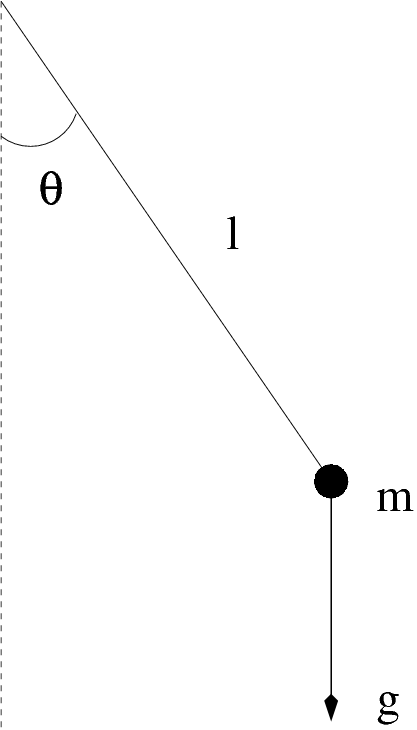


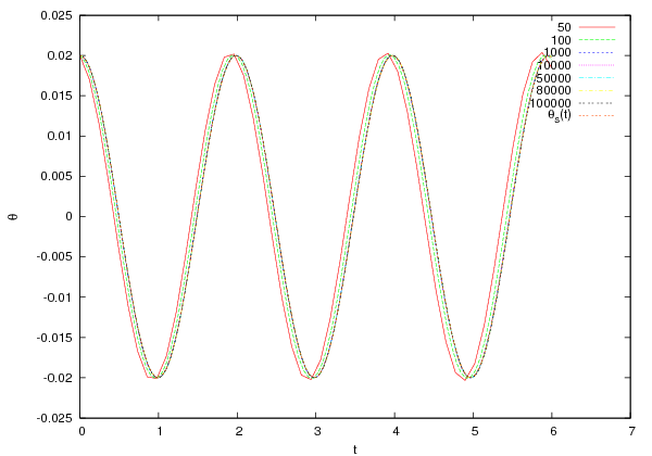
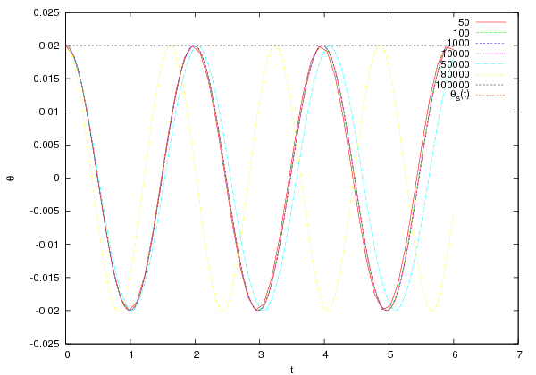


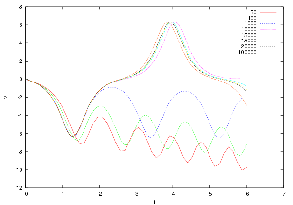


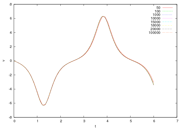
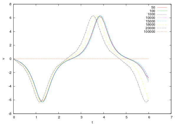


![[ti,tf]](main_latex1533x.png) to
to  equal
intervals
 , where
  . The derivatives are
approximated by the relations
  , so that
 is the angular acceleration. This is the so-called
 .
This is most easily seen by Taylor expanding around the point
  and neglecting all terms starting from the second derivative and
beyond
 ! We expect that errors accumulate in an
additive way at each integration step, and since the number of steps is
 the total error should be
  . This is indeed
what happens, and we say that Euler’s method is a first order method. Its range
of applicability is limited and we only study it for academic reasons. Euler’s
method is
  . It can be put in a more balanced form by using
the velocity
  . This way we obtain the
Euler-Cromer method with a slightly improved behavior, but which is still of first
order
 . This is given by the equations
 . We make one Euler time step
  . If the initial conditions are
  ,
,  , then we

 ,
otherwise it will spoil and eventually dominate the
  total error of the
method introduced by the intermediate steps. At the last step we also have to
take

 due to roundoff errors. In particular, the
second equation in (
 , this difference has to be
computed from the last digits of the finite representation of the numbers
  and
and  in the computer memory. The accuracy in the determination of
 decreases until it eventually becomes
  is smaller by a factor
  compared to the
term
  in Euler’s method. At some point, by decreasing
  , we obtain
 and the accuracy of the method vanishes due to the finite
representation of real number in the memory of the computer. When the
numbers
  and
and  differ from each other by more that
approximately sixteen orders of magnitude, adding the first one to the
second is equivalent to adding zero and the contribution of the acceleration
vanishes
 . For
starters we take
  , the angles
  and the angular velocities
  for
for
 . The user determines the time interval for the integration from
 to
to  and the number of discrete times
  and
and  . After this, we call the main integration functions
which take as input the initial conditions, the time interval of the integration and
the number of discrete times
  , the integration in each of the functions is performed in
 . The results are stored at each
step in the arrays
  . The
Euler–Verlet method converges much faster, but roundoff errors kick in soon.
This is more obvious in figure
  ):
): 
 where the methods converge. This way we can check our program
for bugs. The plot of the functions above can be done with the following
  axis and the value found in the second column
minus the value of the function
  equal to the value found in
the first column on the
  axis. This way, we can make the plots shown
in
axis. This way, we can make the plots shown
in![[ti,tf]](main_latex1594x.png) by
by  discrete times is of order
  , where
 is the time step of the integration. In this section we will
discuss a generalization of this approach where the total error will be of higher
order in
  . This is the class of Runge-Kutta methods which are one step
algorithms where the total discretization error is of order
  . The
local error introduced at each step is of order
  leading after
 steps to a maximum error of order

 order.
The
 .
.
 which evolves in time according to the differential equation:

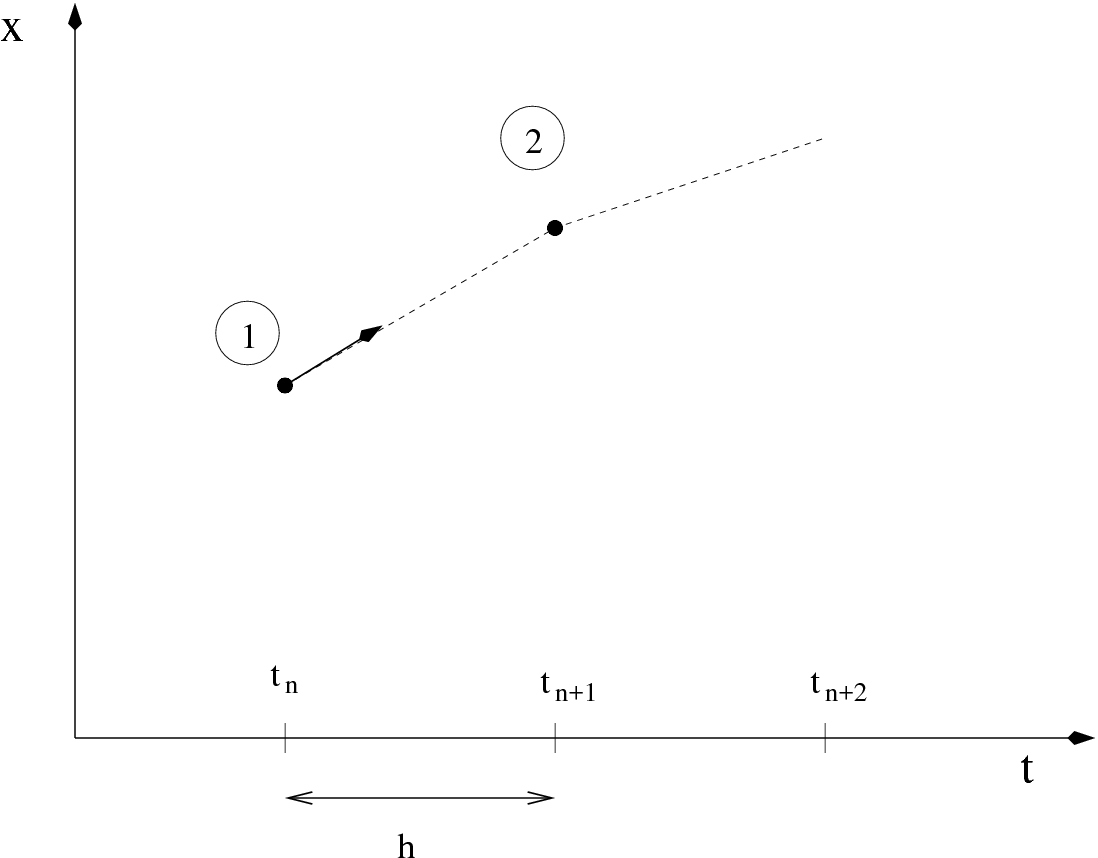


 , therefore the
error after integrating from
  is
is  . Indeed,

 we
determine the point
  .
.
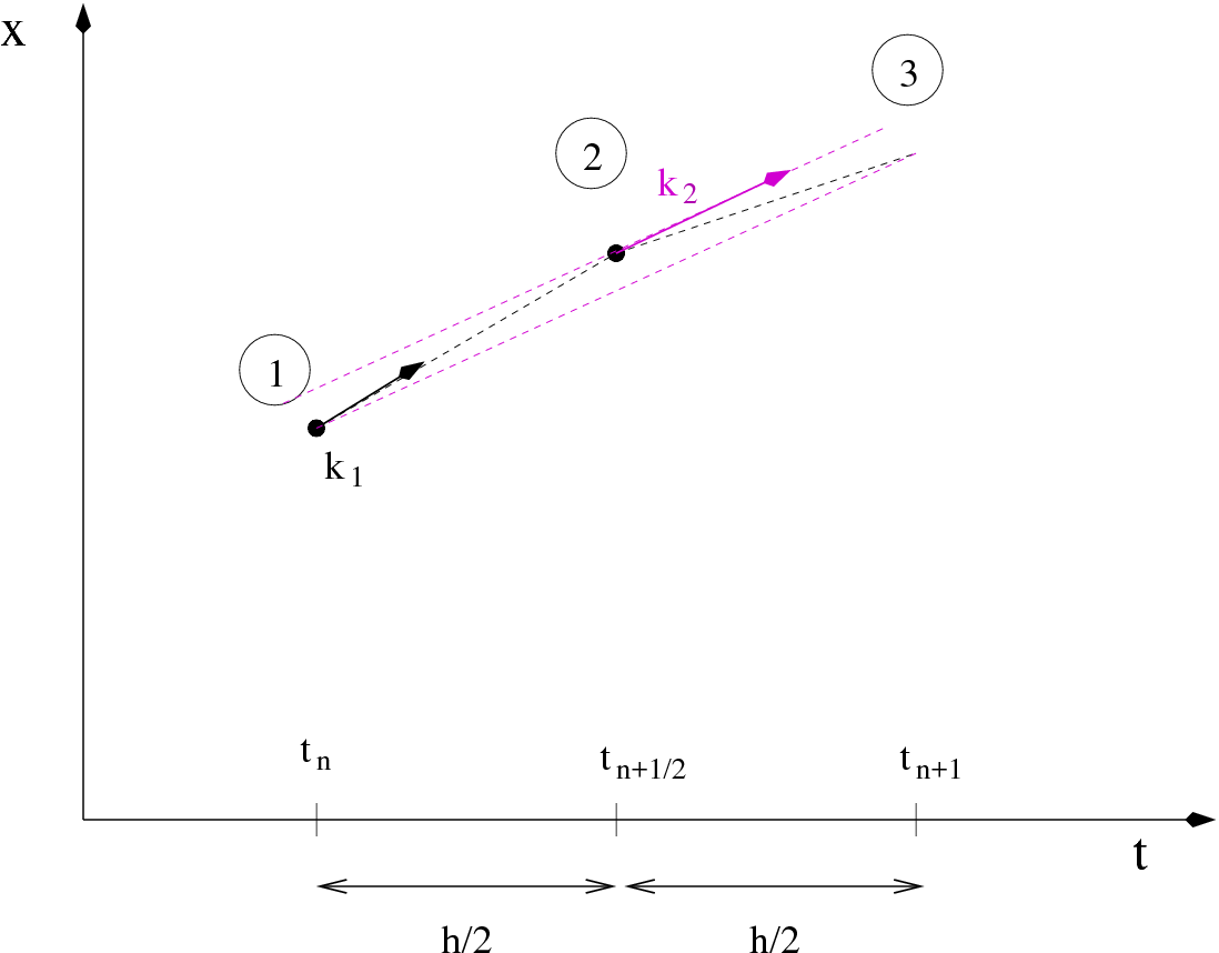
 by making a linear extrapolation from
 in the direction of the derivative
  . Then we use the
slope at point 2 as an
  . We use
  to linearly
extrapolate from
  to
to  . Summarizing, we have that
 twice at each step,
thereby doubling the computational effort. The error at each step (4.19) becomes
 , however, giving a total error of
  . So for given
computational time, (4.19) is superior to (4.17) .

 per step, but the
total error becomes now
  and the method is superior to that of (
 to
to  . Point 2 is
determined by linearly extrapolating from
  to the midpoint of the
interval
  by using the direction given by the derivative
 , i.e.
  . We calculate the derivative
 at the point 2 and we use it in order to determine
point 3, also located at the midpoint of the interval
  . Then we calculate
the derivative
  at the point 3 and we use
it to linearly extrapolate to the
  , thereby
obtaining point 4, i.e.
  . Then we calculate the derivative
 at the point 4, and we use all four derivative
  and
and  as estimators of the derivative of the function in the interval
 . If each derivative contributes with a particular weight in this
estimate, the discretization error can become
  . Such a choice is

 ,
,  ,
,  and
and  respectively. A generic small
change in these values will increase the discretization error to worse than
 .
.
 the discretization
errors decrease, but that roundoff errors will start showing up for small enough
 . Therefore, a careful determination of
  that minimizes the total error
should be made by studying the dependence of the results as a function of
 .
.
 and
and  so
that


 and the corresponding values of the functions
 and
and  ,
,  . The main program calls the driver routine

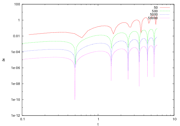


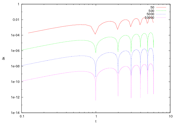

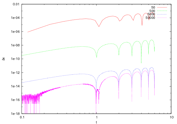


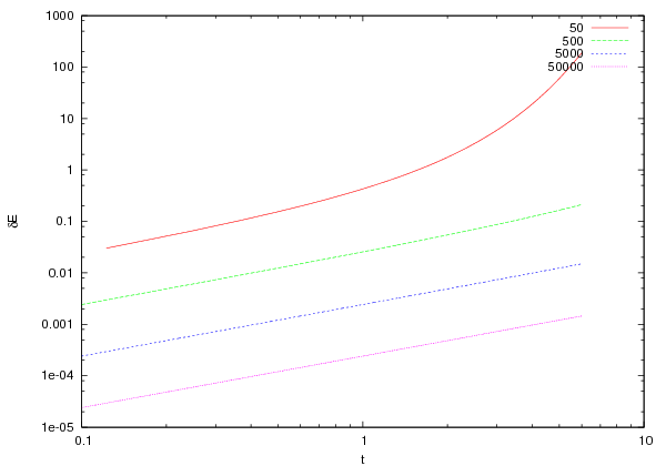

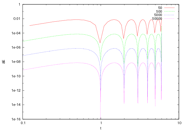
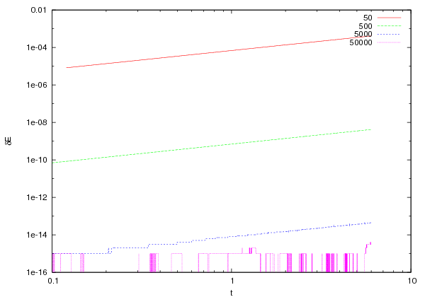
 . We will take
  (
( ). Therefore the relevant part of the program in
  to
to  with the
initial conditions
  ,
,  . The time step
  is varied by
varying the number of steps
 and
and  as a
function of the time step
  . The results are shown in figures 4.11–4.14. We
note that for the Euler method and the Euler–Cromer method, the errors
are of order
  as expected. However, the latter has smaller errors
compared to the first one. For the Euler–Verlet method, the error turns out
to be of order
  whereas for the 4th order Runge–Kutta is of
order
 .
.

 is shown in figures

 and
and  is the angular frequency of the driving
force.
 . The real solutions of the differential
equation
 are given by


 case, the general solution is obtained from the sum of a special
solution
  and the solution of the homogeneous equation
  . A special
solution can be obtained from the ansatz
  ,
which when substituted in (
 and
and  we find
that
![a0 [(ω2 − ω2 )cosωt + γ ωsin ωt]
xs(t) = ------0--2----2-2----2-2-------,
(ω 0 − ω ) + ω γ](main_latex1716x.png)

 decreases exponentially with time and eventually only
 remains. The only case where this is not true, is when we have
resonance without damping for
  ,
,  . In that case the solution
is

 ,
,  ,
,  ,
,  are entered interactively by the user from the standard input
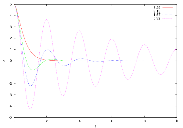


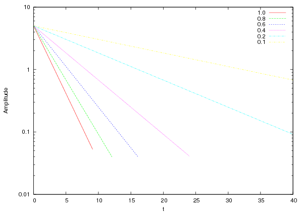


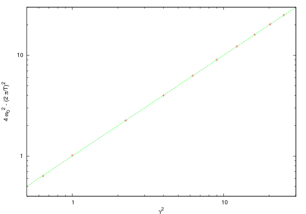


 to an oscillating motion with damping
amplitude for
  . The exponential decrease of the amplitude is shown in
figure
  from the damping coefficient
 is shown in figure
 . The period
  can be estimated from the
time between two consecutive extrema of
  or two consecutive zeros of the
velocity
  (see figure
  to the point
  , independently of the
initial conditions. Such a point is an example of a system’s
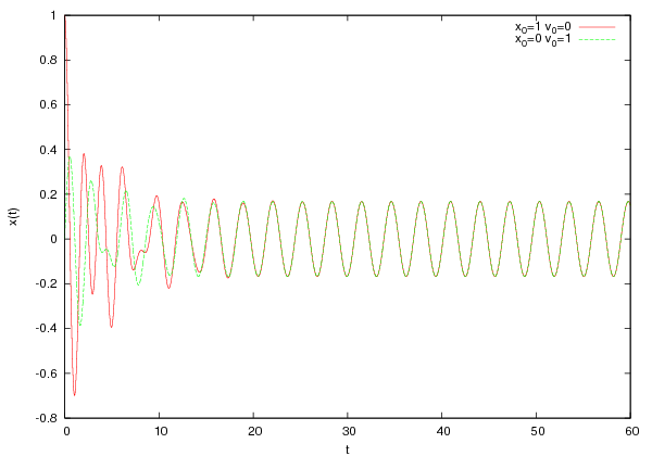


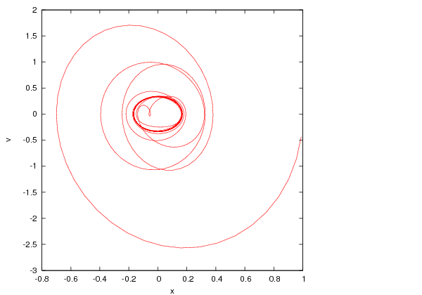


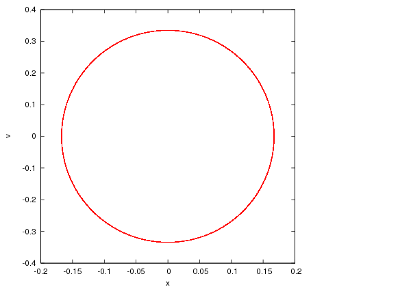

 becomes dominant when
the exponentials have damped away.
  can be written in the form

 on the angular frequency of the driving force. Finally we study
the trajectory of the system in phase space. As we can see in figure 4.20, this time
the attractor is an ellipse, which is a one dimensional curve instead of a zero
dimensional point. For large enough times, all trajectories approach their
attractor asymptotically.

 is the angle of the pendulum with the vertical axis,
  is the damping coefficient,
  is the pendulum’s natural angular
frequency,
  is the angular frequency of the driving force and
  is
the amplitude of the external angular acceleration caused by the driving
force.
 , which is an attractor for the system. This continues
to happen for small enough
  , but for
  the behavior of the system
becomes more complicated.
 ,
,  ,
,  . The final program can be found in the file
 ![[− π,π]](main_latex1783x.png) .
.
 ,
,  , and
, and
 unless we explicitly state otherwise. The natural period of the pendulum
is
  whereas that of the driving force is
 . For
. For  , with
  , the
point
  is an attractor, which means that the pendulum eventually
stops at its stable equilibrium point. For
  the attractor is a
closed curve, which means that the pendulum at its steady state oscillates
indefinitely without circling through its unstable equilibrium point at
  .
The period of motion is found to be twice that of the driving force. For
 the attractor is an open curve, because at its steady state the
pendulum crosses the
  point. The period of the motion becomes
equal to that of the driving force. For
  we have
  , but the trajectory is still periodic. For
even larger values of
 the system enters into a chaotic regime where
the trajectories are non periodic. For
  we find the system in a
periodic steady state again, whereas for
  –
–  we have period
doubling. For
  we enter into a chaotic regime again etc. These
results can be seen in figures
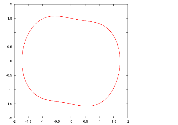
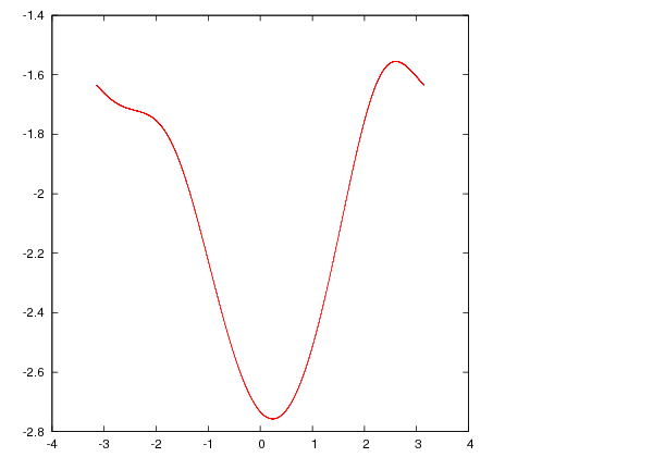


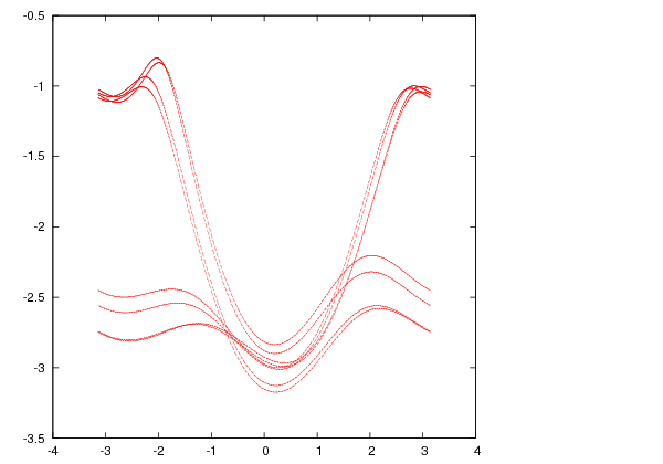
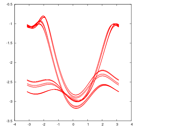
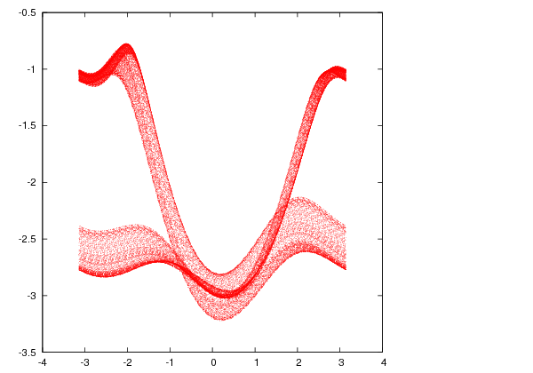


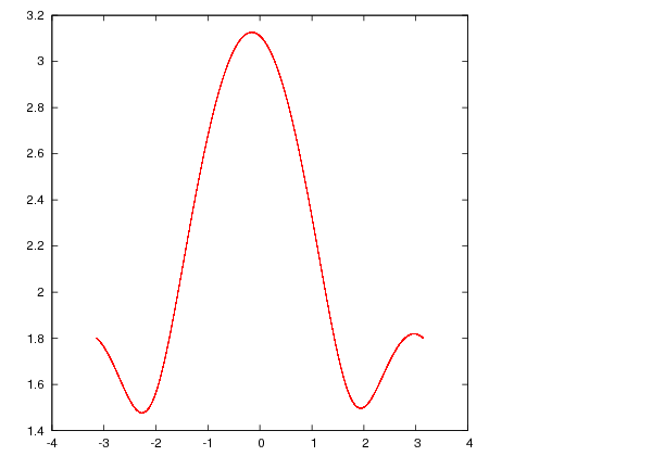
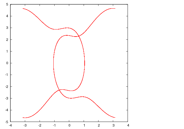
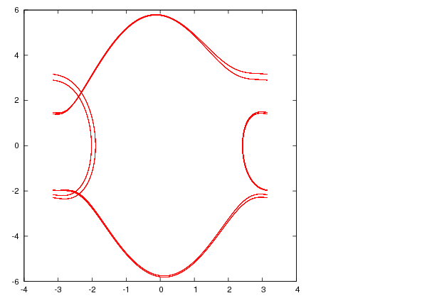
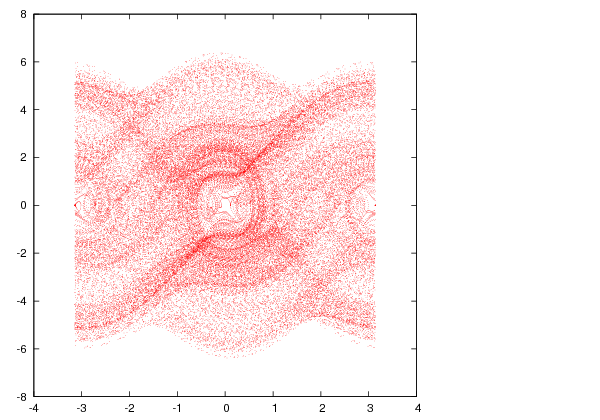


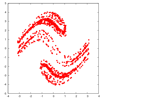
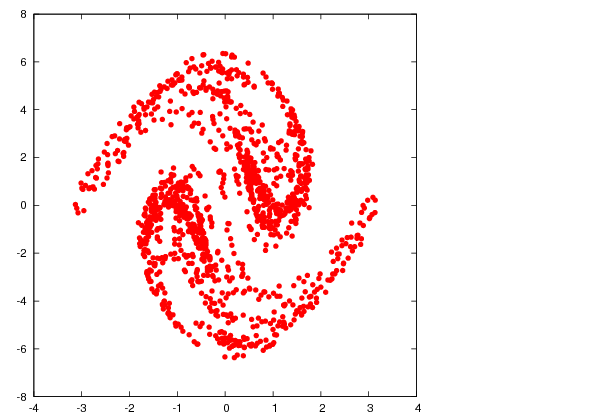


 –multiple of the period of
the driving force then the Poincaré diagram consists of only
  points.
Therefore, in the period doubling regime, the points of the Poincaré diagram
double at each period doubling point. In the chaotic regime, the Poincaré
diagram consists of an infinite number of points which belong to sets that
have interesting fractal structure. One way to construct the Poincaré
diagram numerically, is to process the data of the output file
  ,
the number of points of time and the final time
  . We calculate
the period
  in the regime where the pendulum at its steady
state has a circular trajectory with a positive or negative direction. By
taking a large sample of initial conditions and recording the direction of
the resulting motion after the transient behavior, we obtain figure
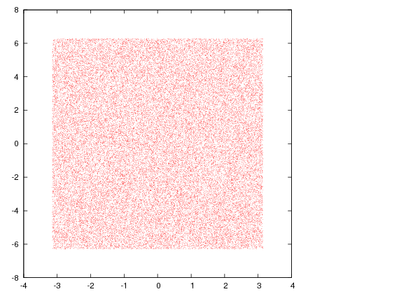


 integration steps. In this method, these errors must be
studied carefully:
  does not accumulate because it is given
by the
  .
.
 is the
  to
to  . Then according to the expansions
(
 .
Then


 , we obtain


 .
.

 which should depend only on the
position
  and not on the velocity.
 . This choice is special, since
by choosing another point (e.g.
  ) the result would have not been the
same. Indeed, from the relation
 we obtain


 term it is necessary to place the
intermediate point at time
  .
.
 we obtain
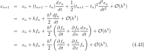
 ,
,  etc. We define
 of the last
equation in the error are identical with those of equation (4.43) . By expanding
 we obtain
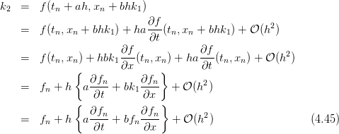


 ,
,  ,
,  leads to equation (4.19) . Some other
choices in the bibliography are
  and
and  .
.
 .
.
 ,
,  ,
,  .
.
 on the particle. Consider the
case
  ,
,  ,
, 
 . Calculate the
limiting velocity of the particle numerically and compare the value
obtained to the theoretical expectation.
 .
.
 ,
,  and calculate its mechanical energy as a
function of time. Is it monotonic? Why? (show that
  ).
Repeat for
  . When is the system oscillating and when it’s
not? Calculate numerically the critical value of
  for which the system
passes from a non oscillating to an oscillating regime. Compare your results
with the theoretical expectations.
 numerically and compare with equation (
 . Define “momentary” to be an impulse given by the
acceleration
  by an appropriately small time interval
  . The
acceleration is
  for all other times. Calculate the amplitude
  for
for
 and
and  .
.

 and
and  . Calculate
the amplitude
  .
.

 and
and  . Calculate
the amplitude
  . Compare your results with those of the previous
problem and comment about.
 identical, independent harmonic
oscillators. Take
  and choose random initial conditions for each one
of them. Study their trajectories in phase space and check whether they
cross each other. Comment on your results.
 harmonic oscillators of the previous problem in a
small square in phase space whose center is at the origin of the
axes. Consider the evolution of the system in time. Does the shape
of the rectangle change in time? Does the area change in time?
Explain...
 .
Take
  .
.
 ,
,  ,
,  .
Study the transient behavior of the system in the plots of
  ,
,  for
for
 .
.
 ,
,  ,
,  and study the phase space trajectories for
  0.1, 0.19, 0.21, 0.25, 0.5,
0.71, 0.79, 0.85, 1.02, 1.031, 1.033, 1.05, 1.08, 1.1, 1.4, 1.8, 3.1, 3.5, 3.8, 4.2,
4.42, 4.44, 4.445, 4.447, 4.4488. Consider both the transient behavior and
the steady state motion.

 ,
,
 and
and  is periodic. Measure the period of the
motion with an accuracy of three significant digits and compare it
with the natural period of the pendulum and with the period of the
driving force. Take as initial conditions the following pairs:
 ,
,  ,
,  ,
,  ,
,  ,
,  ,
,
 ,
,  . Check if the period is independent of the initial
conditions.

 takes values in
the interval
 ![[0.2,5.0]](main_latex1937x.png) . Consider specific discrete values of
. Consider specific discrete values of  by splitting
the interval above in subintervals of width equal to
  .
For each value of
  , record in a file the value of
  , the angular
position and the angular velocity of the pendulum when
  with
with
 :
:

 is made so that the transient behavior will be
discarded and study only the steady state of the pendulum. You
may take
  ,
,  ,
,  ,
,  , and
split the intervals
 ![[tk,tk + π]](main_latex1950x.png) to 50 subintervals. Choose
to 50 subintervals. Choose  ,
,
 .
.
 .
.
 .
.
 ,
,  .
Repeat your analysis for
  ,
,  .
.
![A ∈ [1.0000,1.0400]](main_latex1959x.png) with
with
 and
and ![A ∈ [4.4300,4.4500]](main_latex1961x.png) with
with  and
compute with the given accuracy the value
  where the system
enters into the chaotic behavior regime.
 for
for 


 . Put 2000 points for each value of
  and
commend on the strength of the chaotic behavior of the pendulum.
 etc.
etc.
 ,
,  ,
,  ,
,  , and the values of the functions of
time will be stored in the arrays
  ,
,  ,
,  ,
,  . The integration is performed by a call to the
function
  so that


 is the direction of the initial velocity and
  is the
maximum height of the trajectory.
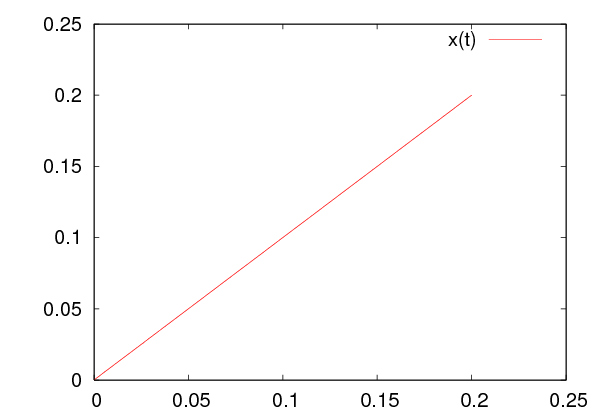
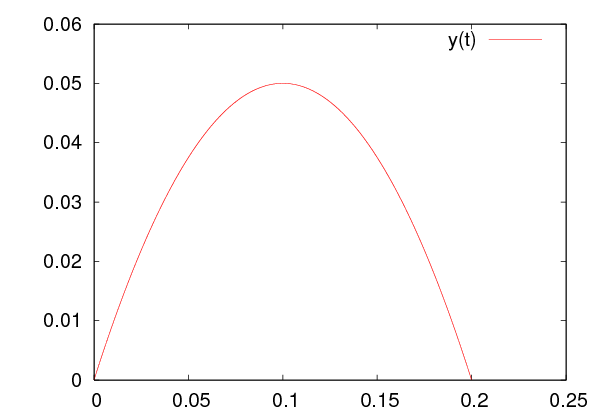
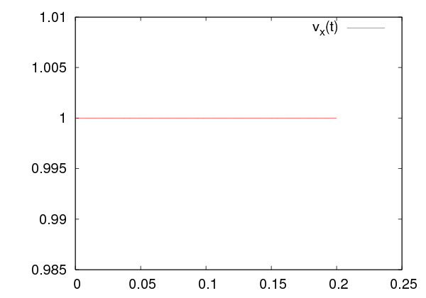
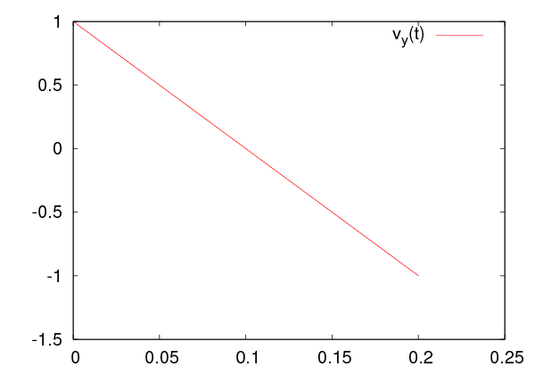


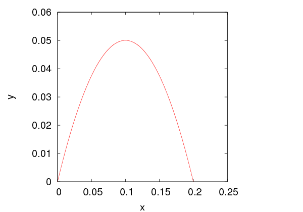
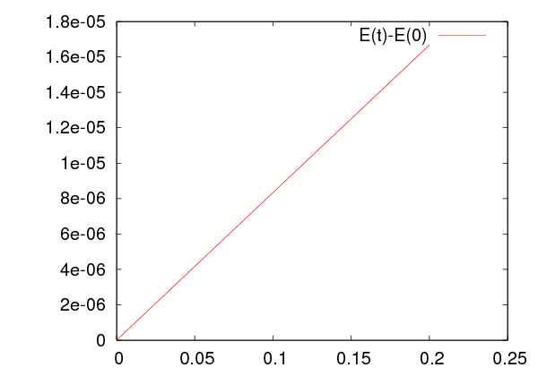


 (
(

 , the coordinate
  etc. The keyword
  ,
,
 ) and the scattering of a particle in a Coulomb field –
try them! I hope that you will have enough curiosity to look “under the
hood” of the scripts and try to modify them or create new ones. Some
advise to the lazy guys: If you need to program your own force field follow
the recipe: Write the code of your acceleration field in a file named e.g.
 , therefore

 (
( const.,
  ).
).
 ,
,  )
)  is shown in figure
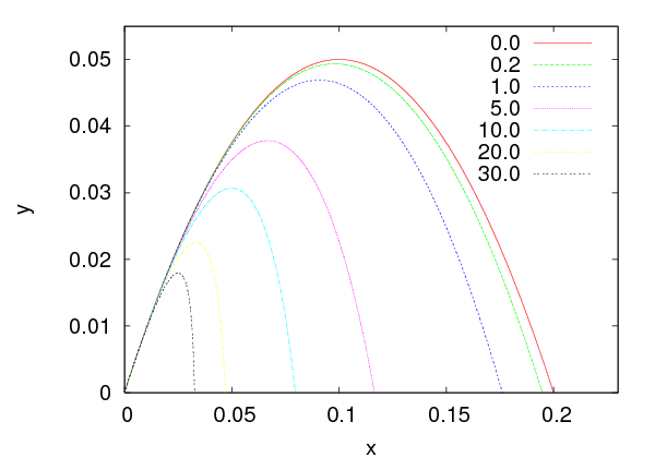
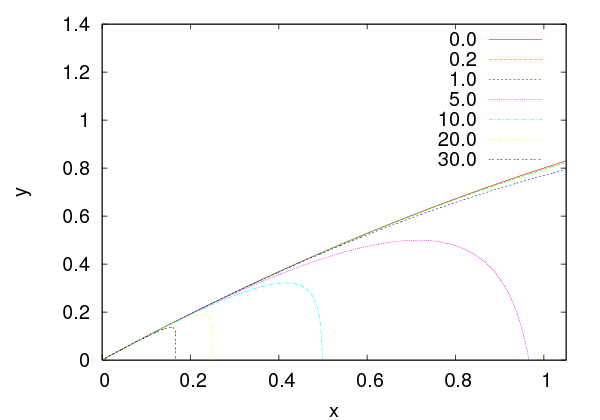


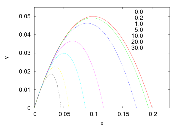


 and a planet “earth”
at distance
  from the sun and mass
  such that
  . According to
Newton’s law of gravity, the earth’s acceleration is
 ,
,  ,
,  .
When the hypothesis
  is not valid, the two body problem is reduced to
that of the one body problem with the mass replaced by the reduced mass


 with respect to the center of the force, which in turn
implies that the motion is confined on one plane. We choose the
  axis so
that


 . This is a system of two coupled differential equations for the
functions
  ,
,  . The trajectories are conic sections which are either an
ellipse (bound states - “planet”), a parabola (e.g. escape to infinity when the
particle starts moving with speed equal to the escape velocity) or a hyperbola
(e.g. scattering).
 of a
planet satisfies the equation

 is the semi-major axis of the elliptical trajectory. The eccentricity is a
measure of the deviation of the trajectory from being circular
 is the semi-minor axis. The eccentricity is 0 for the circle and tends to 1
as the ellipse becomes more and more elongated. The foci
  and
and  are
located at a distance
  from the center of the
 and take special care to avoid hitting the center of the
force, the singular point at
  . The same code can be used for the
electrostatic Coulomb field with
  .
.
 ,
,
 ,
,  ,
,  and vary
  . We measure the period
  and
the length of the semi axes of the resulting ellipse. The results can be found in
table


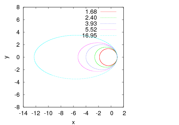


 lie on a straight line. Using a linear least
squares fit we calculate the slope and the intercept which should be equal to
  and
and  respectively. This is left as an exercise.
 , the particle escapes from the influence of the gravitational
field to infinity. The escape velocity corresponds to zero mechanical energy, which
gives

 ,
,  ,
,  , we obtain
  . The
numerical calculation of
  is left as an exercise.

 . Scattering problems are interesting because we can
infer to the properties of the scattering potential from the distribution of
the scattering angle. This approach is heavily used in today’s particle
accelerators for the study of fundamental interactions between elementary
particles.
 by other hard spheres or radius
  . The interaction
potential
 is the distance between the center of
  from the center of
  .
.
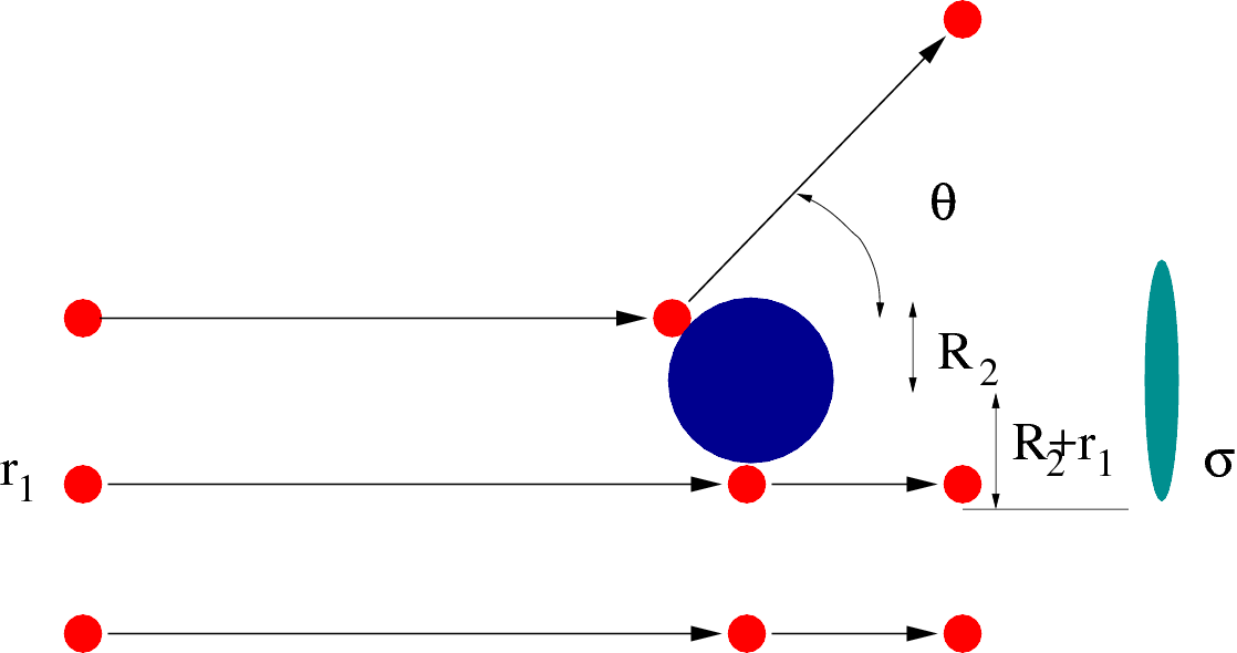


 be the intensity of the
beam
 its cross sectional area. Assume that the target has
  particles per unit
area. The cross sectional area of the interaction is
  where
where  and
and  are the radii of the scattered particles and targets respectively (see figure
(
 is the total number of target spheres which lie within the beam. On
the average, the scattering rate is
 of the interaction. The differential cross section
  is defined by the
relation
 is the number of particles per unit time scattered within the solid
angle
  .
. 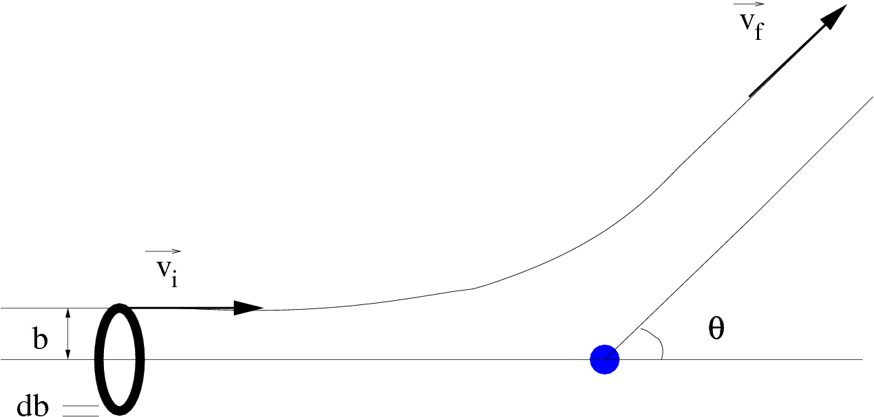


 and
and
 . This is the relation that we will use in the numerical calculation of
 .
.
 depends on the
impact parameter
  .
. , thickness
  and area
  is scattered in angles between
  and
and  . Since there is only one particle at the target we have that
 . The number of particles per unit time crossing the ring is
  ,
therefore

 sign is because as
  increases,
  decreases). From the potential we can
calculate
  and from
  we can calculate
  . Conversely, if we measure
 , we can calculate
  .
.
 (“electron”) in a
Coulomb potential of a much heavier charge
  (“nucleus”) is called
Rutherford scattering. In this case, the interaction potential is given by


 and the magnitude of its angular
momentum is
  , where
  . The dependence of the impact parameter
on the scattering angle is


 where the scattering angle is
  . A large number of integration steps
is needed in order to obtain the desired accuracy. A useful monitor of
the accuracy of the calculation is the measurement of the energy of the
particle which should be conserved. The results are shown in table


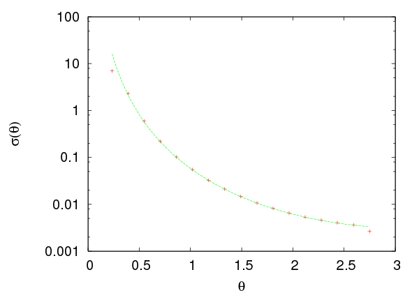


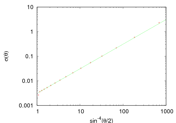


 and
and  . For this reason we split the interval
 ![[0,π ]](main_latex2326x.png) in
in  bins
so that
  . We perform “scattering experiments” by varying
![b ∈ [bm,bM ]](main_latex2329x.png) with step
with step  . Due to the symmetry of the problem we fix
  to be a constant, therefore a given
  corresponds to a cone with an
opening angle
  and an apex at the center of scattering. For given
  we
measure the scattering angle
  and record the number of particles per unit
time
  . The latter is proportional to the area of the ring of
radius
  . All we need now is the beam intensity
  which is the total
number of particles per unit time
  (note than in the ratio
 the proportionality constant and
  cancel) and the solid angle
 . Finally we can easily use equation (
 . The program that performs this calculation is in
the file
 by the
hydrogen atom. The positron has positive charge
  and the hydrogen atom
consists of a positively charged proton with charge
  in an electron
cloud of opposite charge
  . We set the scales so that
  and
and
 . We will perform a numerical calculation of
  ,
,  and
and
 .
.

 for
for  . The program containing the calculation of the
acceleration caused by this force can be found in the file
  (see
problem 5.


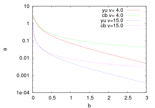


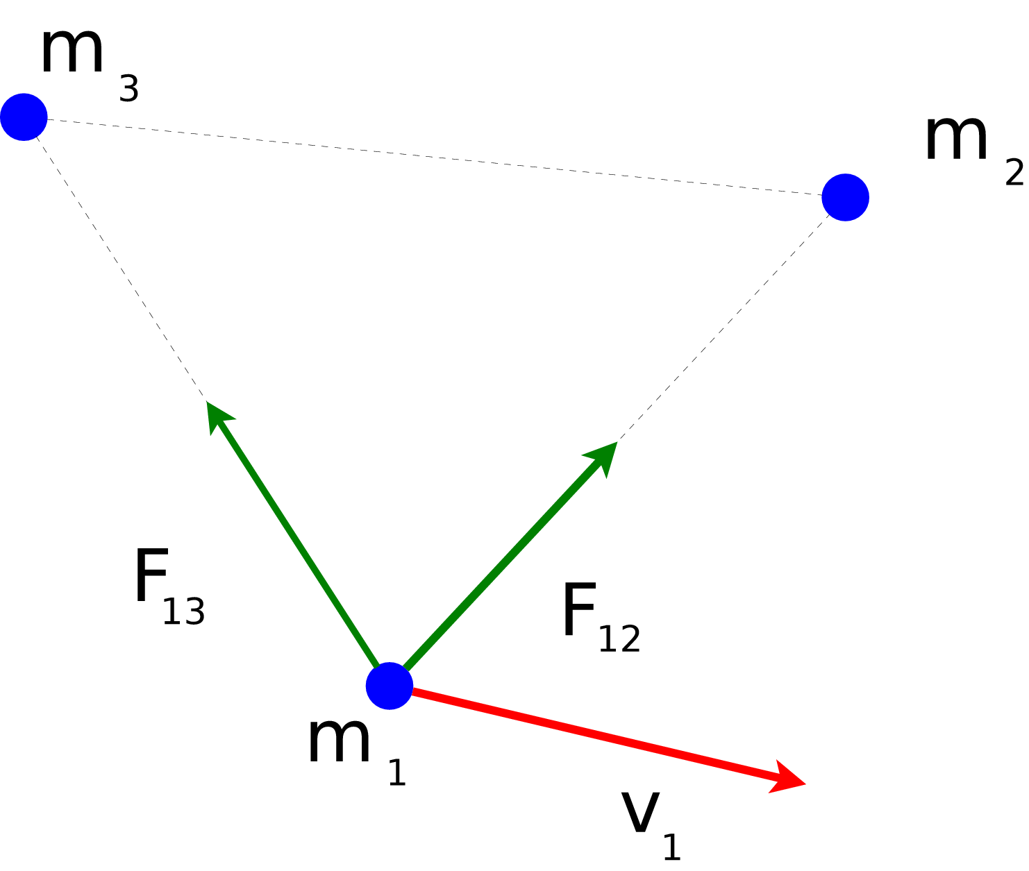

 and the equations of motion become (
 )
)

 . The total energy of the system is

 ,
,  ,
,  ,
,
 ,
,  ,
,  ,
,  ,
,  and
and  .
.
 and compute its trajectory for
 . Set
. Set  and calculate the
resulting radius of the trajectory. Plot the relation between the radius
and
  . Compare your results to the known analytic solution. (assume
non relativistic motion)
 ,
,  . Construct the Lissajous
curves by setting
  ,
,  ,
,
 ,
,  . What happens when
  ?
?
 vs
vs  and calculate the slope of the resulting straight
line by using the linear least squares method. Is it what you expect?
Calculate the intercept and compare your result with the expected one.
 for
for  ,
,
 ,
,  using the following steps: First show
that
  . Then set
  ,
,  . Vary
 and measure the resulting semi-major axis
  . Determine
the intercept of the resulting straight line in order to calculate
  .
.
 ,
,  ,
,  ,
,  ,
,  ,
,
 ,
,  ,
,  . From the
  plot confirm the relation
(
 ,
,
 ,
,  ,
,  ,
,  you obtain that
 for each point
  of the trajectory. The point
  is the center of the force. After determining the semi-major axis
  numerically, the point
  will be taken symmetric to
  with respect
to the center of the ellipse.
 and
and  for
different values of
  . Calculate the total cross section
  numerically
and show that it is equal to
  .
.

 . Compute the solutions of the problem numerically in one
dimension and compare them to the known analytic solutions when
 :
:

![[ αx0 ]
C = sin−1 ∘D--−-|E|e----- .
D(D − |E|)](main_latex2457x.png)
 . For
. For  we obtain


 is given by a different
relation and not by equation (
 and study the transition from open to closed trajectories.
 (
( ) in the
previous problem. Plot the function
  for
for  ,
,
 ,
,  ,
,  , and of course for
  . Determine the
equilibrium position and the ionization energy.
 ,
,  ,
,  ,
,  on the plane for
  ,
,
 , and
, and  numerically. In the
  case consider the scattering
problem and calculate the functions
  ,
,  and the total cross section
 .
.
 where
where  . Calculate the potential
 and plot the function
  . Determine the
equilibrium position and the ionization energy.
 ,
,  and
and  numerically. How much do your results depend on the minimum scattering
angle?
 . Determine appropriate initial conditions that give a spiral
trajectory.
 for the Rutherford scattering both
analytically and numerically. What happens to your numerical results as you
vary the integration limits?
 static point
charges.
 plane in a constant magnetic field
  . Solve the equations of motion
using a 4th order Runge–Kutta Method. Plot the resulting trajectories for
the initial conditions that you will choose.
 are connected by identical springs. The
springs’ spring constant is equal to
  and their equilibrium length is equal
to
  . The particles move without friction on a horizontal plane. Solve the
equations of motion of the system numerically by using a 4th order
Runge–Kutta Method. Plot the resulting trajectories for the initial
conditions that you will choose. (Hint: Look in the files
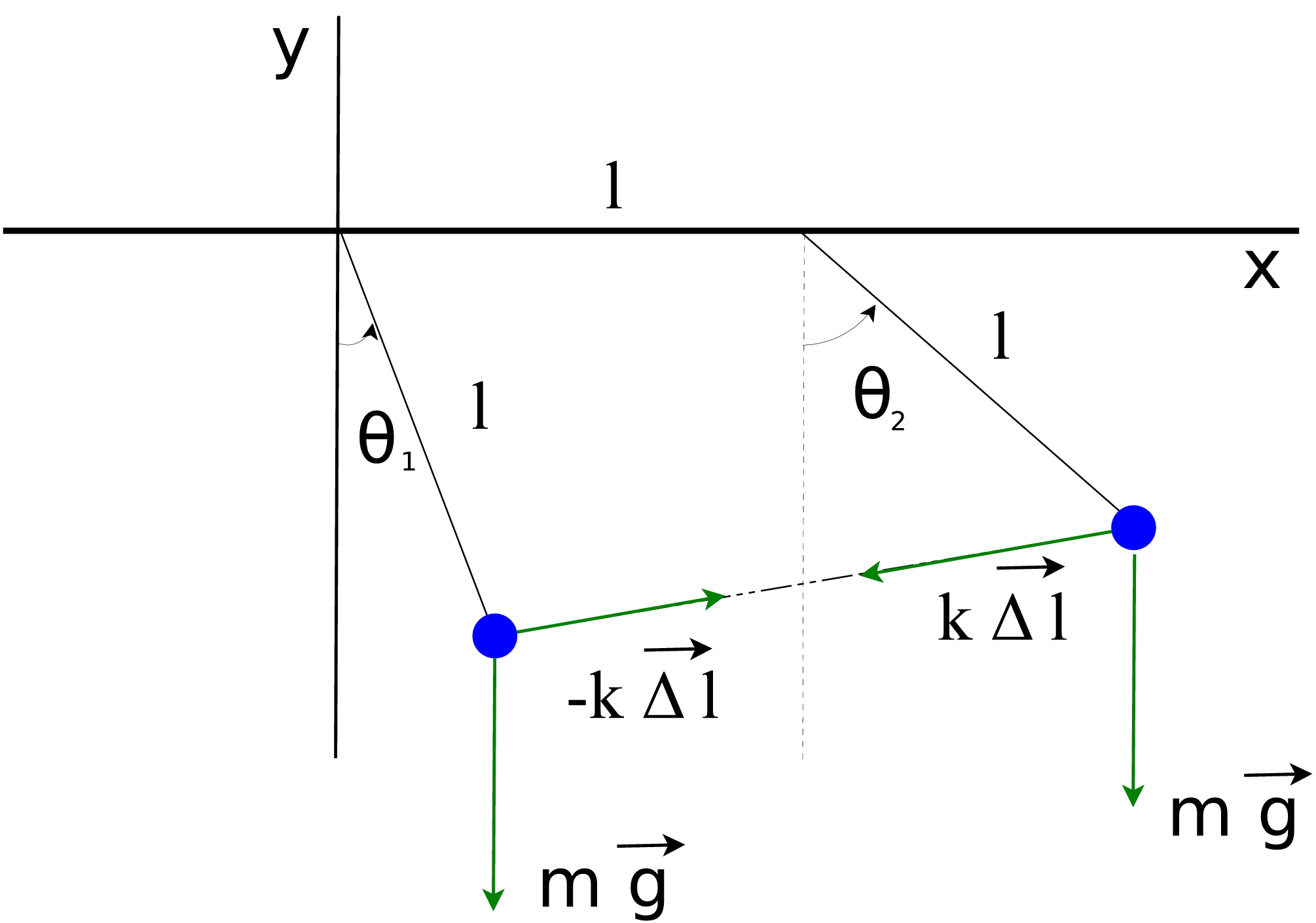


 and they are connected by an ideal weightless spring with spring
constant
  and equilibrium length
  . The rods are hinged to the
ceiling at points whose distance is
  (see figure
  and
and  . Solve these equations numerically by
using a 4th order Runge–Kutta method. Plot the positions of the
particles in a Cartesian coordinate system and the resulting trajectory.
Study the normal modes for small angles
  and compute the
deviation of the solutions from the small oscillation approximation as
the angles become larger. (Hint: Look in the files
  axis.
axis.
 .
.
 and one of order
  , and the difference of the results
is used as an estimate of the truncation error. If the error needs to be
reduced, the step size is reduced and if it is satisfactorily small the step
size is increased. For the details we refer the reader to


 . The first three
positions are the coordinates of the initial position and the last three
the components of the initial velocity. Then, we set some variables that
determine the behavior of the integration program (see the file
  =
=  =
=  =
=  =
=  =
=
 =
=  we end the
calculation.
 . The program is in the file
 and
and 

 ,
,  .
The components of the acceleration of the particle are:
 ,
,  ,
,  and
and  :
:
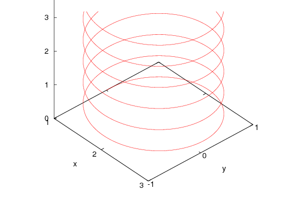


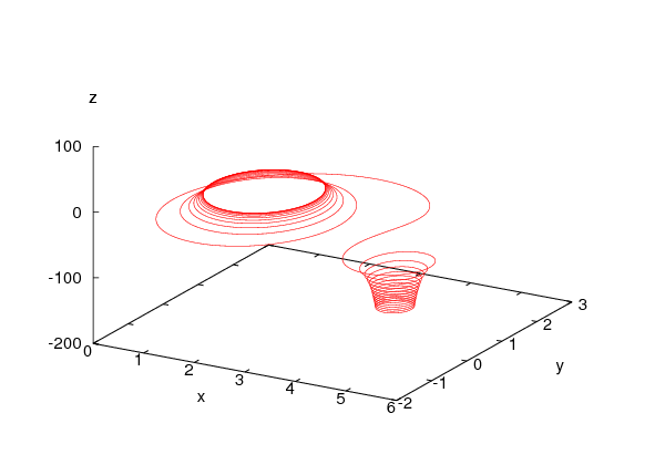


 with
with
 ,
,  and
and  ,
,  .
Note that
  . You may also want to calculate the current density from
the equation
  .
.
 . The particle’s rest mass is
  , its
mass is
  (where
  ), its momentum is
  and its
energy is
  . Then the equations of motion in a dynamic field
 are given by:


 we obtain


 . Given the initial conditions


 their solution is
unique and it can be computed numerically using the 4th-5th order Runge–Kutta
method according to the discussion of the previous section. By using the relations
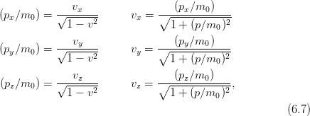
 ,
,  ,
,  ,
,  ,
,  ,
,  instead. Similarly, from the solutions
  ,
,  ,
,  ,
,  ,
,
 ,
,  we can calculate
  ,
,  ,
,  ,
,  ,
,  ,
,
 . We always have to check that


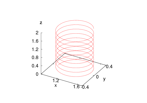


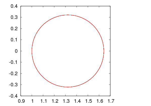


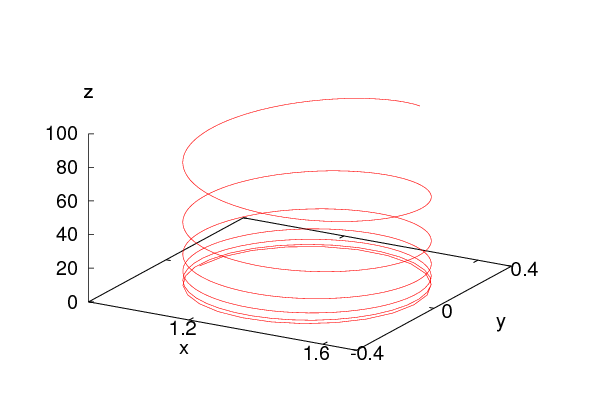

![( )3 [ ]
B⃗ = B0 RE-- 3 (dˆ⋅ ˆr)ˆr − ˆd ,
r](main_latex2634x.png)
 is the magnetic dipole moment of the Earth’s magnetic field and
 . The parameter values are approximately equal to
  ,
,
 , where
  is the radius of the Earth. The typical energy of
the moving particles is
  MeV which corresponds to velocities of
magnitude
  . We choose
the coordinate axes so that
  and we measure distance in
  units
units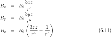
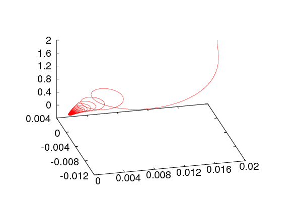


 ,
,  ,
,  . The problem of why the effect is not seen
near the equator is left as an exercise.
 . Assume that their interaction is given by the
Coulomb force only. Write a program that computes their trajectory
numerically using the RK45 method.


 . Compute the
three dimensional Lissajous curves which appear for appropriate
values of the angular frequencies
  ,
,  ,
,
 .
.
 are at the fixed positions
  and
and
 . A third particle of mass
  interacts with them via a
Newtonian gravitational force and moves at non relativistic speeds.
Compute the particle’s trajectory and find initial conditions that result
in a planar motion.
 and
and  .
.
 is given by:
 ,
,  ,
,  and
and
 are the polar coordinates of the point where the electric field is
calculated. Calculate the trajectory of a test charge moving in this
field at non relativistic speeds. Calculate the deviation between the
relativistic and the non relativistic trajectories when the initial speed is
 respectively (ignore radiation effects).
 .
The electric field is given by

 axis. The linear charge density is
  and it is constant. The four straight
lines intersect the
  plane at the points
  ,
,  ,
,  ,
,
 . Calculate the trajectory of a non relativistic charge in this
field. Next, compute the relativistic trajectories (ignore all radiation
effects).
 interact via their Newtonian gravitational force.
Compute their (non relativistic) trajectories in space.
 point charges
  which are located at fixed positions on the plane
given by their position vectors
  ,
,  . The electric field is given by
Coulomb’s law
 is the unit vector in the direction of
  . The
components of the field are
 is
is

 , i.e. the
curves whose tangent lines at each point are parallel to the electric field at that
point. The magnitude of the electric field is proportional to the density of the field
lines (the number of field lines per perpendicular area). This means that the
electric flux
  through a surface
  is proportional to the number
of field lines that cross the surface. Electric field lines of point charge distributions
start from positive charges (sources), end in negative charges (sinks) or extend to
infinity.
 , and it
points in the direction of decreasing
  . The planar cross sections of the
equipotential surfaces are closed curves which are called equipotential
lines.
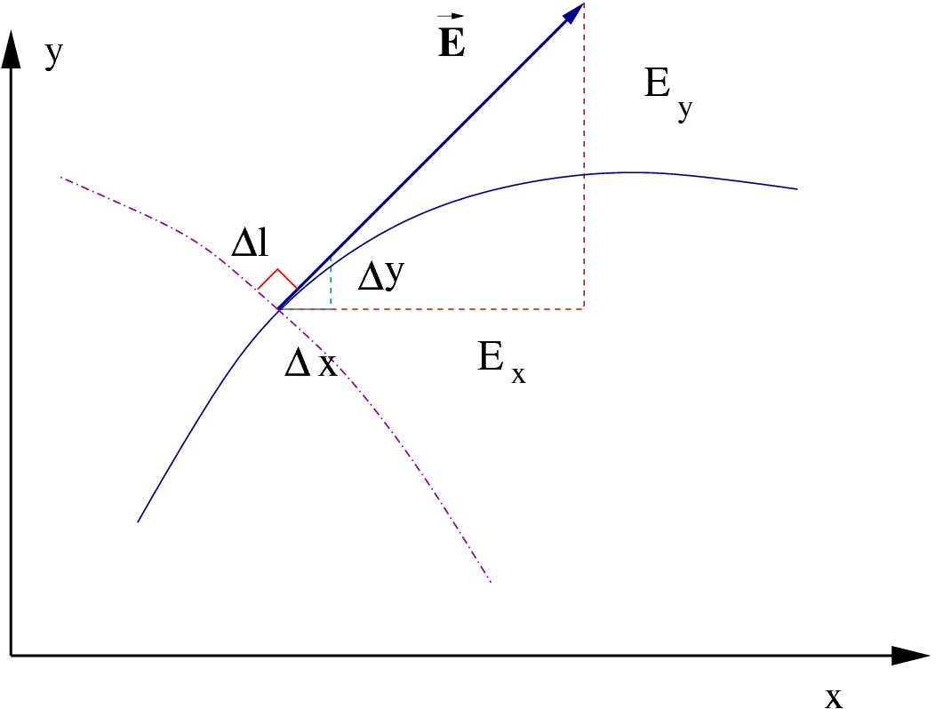


 is taken in the direction of the electric field
and we obtain

 .
.
 is in the
tangential direction of a field line, then
  is in the perpendicular
direction since
  . Therefore the
equations that give the equipotential lines are

 we move in the direction
  to the new
position

 and
and  respectively. The next lines call the function
  ,
,  ,
,
 ,
,  :
:
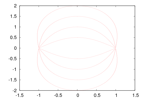
 located at the
origin and we draw one field line passing through the point
  .
.
 below, located at the vertices of a
square:
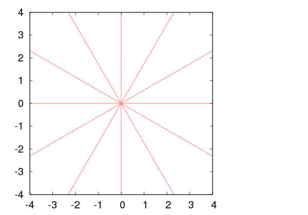
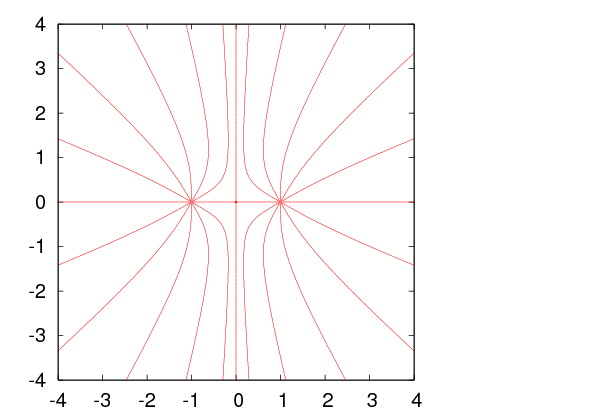

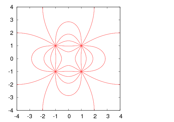
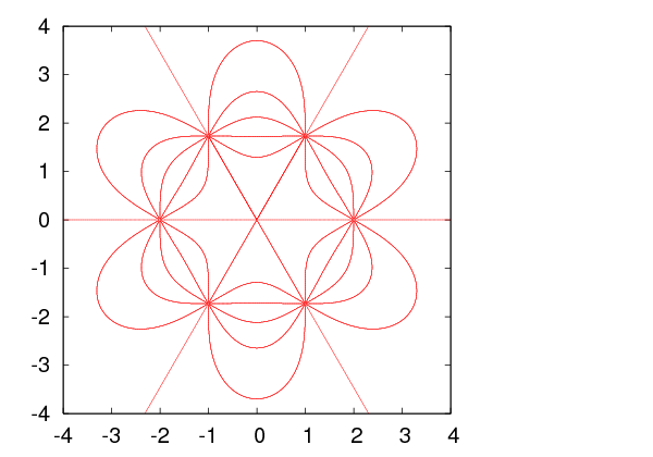
 ,
,
 ,
,  ,
,  (
(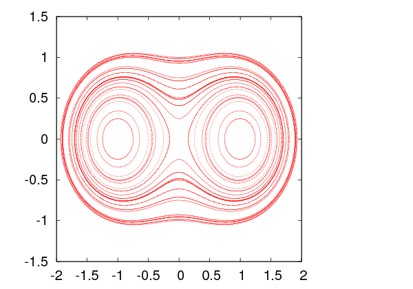
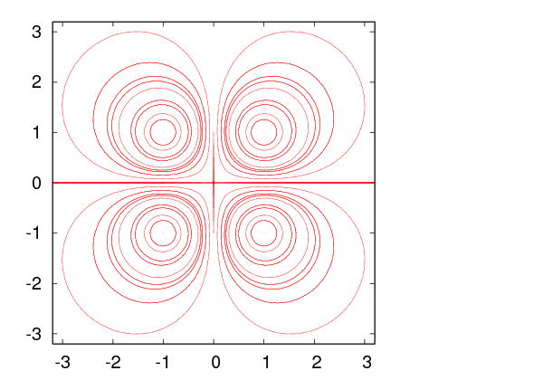
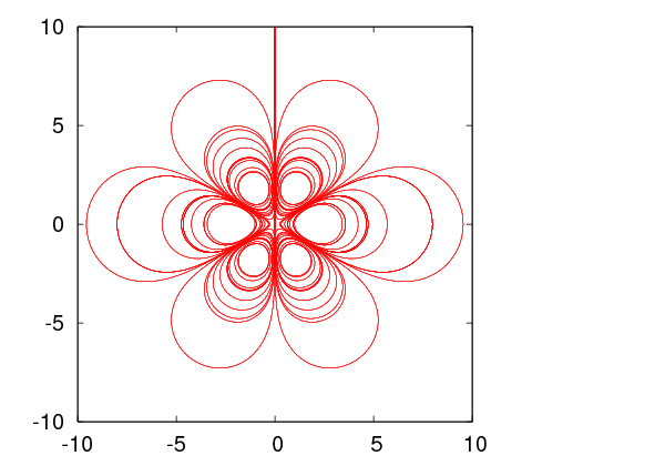
 of equation (
 . The size of the drawing area of the curve is set
by the parameter
  , the motion is in the direction of the electric field,
which ends on a negative charge or outside the drawing area (why?). In
order to draw the line in both directions, set
  and repeat the
calculation.
 ). The
loop is executed twice with
  and
and
 .
.


 :
:

 in a region of space
  bounded by a closed
surface
  . When the potential is known on
  the solution to (
 .
.
 . In this case the last term in equation (
 is a compact subset of the plane and
  is a closed curve.
 by a discrete,
square lattice. The potential is defined on the
  sites of the lattice. We
take
  to be bounded by a square with sides of length
  . The distance
between the nearest lattice points is called the lattice constant
  .
. , where
  is the number of lattice points on each side of
the square. The continuous solution is approximated by the solution on
the lattice, and the approximation becomes exact in the
  and
and
 limits, so that the length
  remains constant. The
curve
  is approximated by the lattice sites that are located on the
perimeter of the square and the loci in the square where the potential takes
constant values. This is a simple model of a set of conducting surfaces
(points where
  const.
  ) in a compact region whose boundary is
grounded (points where
  ). An example is depicted in figure

 according to the equations:
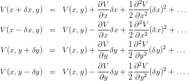
 and ignoring the
terms implied by
  , we obtain
 such that
 and
and  where
where  . By taking
  so that


 and
and 


 , equation (
 is the
arithmetic mean of the potential of the nearest neighbors. We will describe an
algorithm which belongs to the class of “successive overrelaxation methods”
(SOR) whose basic steps are:
 of the square lattice.
 on the vacuum sites. Of
course it is not the solution we are looking for. A good choice will lead
to fast convergence of the algorithm to the true solution. A bad choice
may lead to slow convergence, no convergence or even convergence to
the wrong solution. In our case the problem is easy and the simple
choice
  will do.
 .
. result in
the same solution.
 and the
two conductors are at constant potential
  and
and  respectively. The
user enters the values
  and
and  , the lattice size
  and the required
accuracy interactively. The latter is determined by a small number
  . The
convergence criterion that we set is that the maximum difference between the
values of the potential between two successive sweeps should be less than
 .
.
 with the
 . In this case the Laplace equation becomes the Poisson
equation:

 .
. 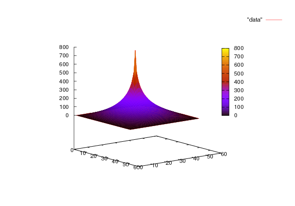

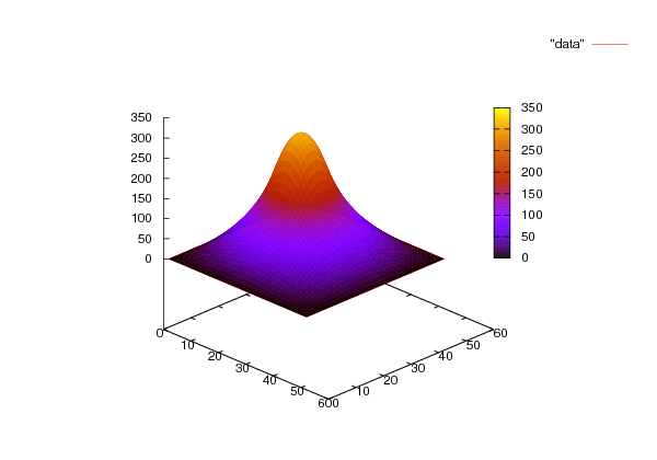

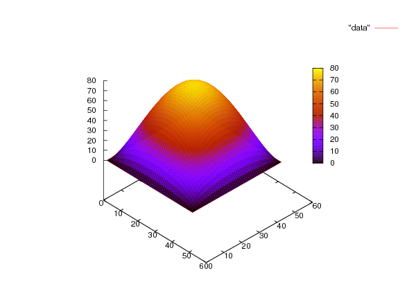

 .
The reader is asked to reproduce this figure together with figures
  and
and  is immediately
updated. In contrast, the Jacobi method uses the
  of equation
(
 is a solution of equation (
 ,
Jacobi’s method can be formulated as

 refer to the values of the potential during
the
  -th sweep. The successive overrelaxation (SOR) method is given
by:
 we have “underrelaxation” and we obtain slower convergence than
the Jacobi method. When
  we have “overrelaxation” and an
appropriate choice of
  can lead to an improvement compared to the Jacobi
method. When
  SOR diverges. Further study of the SOR methods is left as
an exercise to the reader.
 is proportional
to
  .
.
 at the
point
  .
.
 from each other.
 /
/ and use them in order to choose the values
of the potential on the equipotential lines that you plan to
draw. If e.g. you choose to draw 5 equipotential lines, take
 and
and 
 .
.
 chosen in the previous step,
draw an equipotential line from that point.
 .
.
 . Vary
  on
on
 (
( (
(
 of the
system of conductors of the previous problem when
  ,
,  . In
order to calculate the charge
  , compute the surface charge density
  using the equation

 is the perpendicular component of the electric field on the
surface. Use the approximation

 is the potential difference between a point on the conductor and
its nearest neighbor. By integrating (i.e. summing) you can estimate the
total charge on each conductor. If these are opposite and their absolute
value is
  , then the capacitance can be calculated from the equation
 . Perform the calculation described above for
  and
and
 . Verify
that the capacitance is independent of
  . Use
. Use  in the corresponding equations in the
program in the file
  and print the results in the file
  instead of
 . Take
  in the square
 ,
,  . Study the convergence of the solutions by plotting
the section
  for each
  ,
,  ,
,  ,
,  ,
,  ,
,  ,
,  . What happens when
 ?
?
 ,
,  ,
,  ,
,  ,
,  ,
,  ,
,  . What happens when
 ?
?
 at
time
  if the particle is at
  at
at  . The equation that determines
 is
is
 depends on the
details of the system that is studied. For example, for the Brownian
motion of a dust particle in a fluid which moves under the influence of
random collisions with the fluid particles, we have that
  ,
where
  is the (absolute) temperature of the fluid,
  is the friction
coefficient
 is the Boltzmann constant.
 the particle is localized at one
point
  , i.e.
 as a probability density implies that for
  we
should have that
 is normalized so that (
 , the time evolution of
 is governed by equation (
 , then it will hold at all times
if


 and that

 we obtain
 .
.
 for small times is


 of space.
  in our
case.
 is easily
calculated
 so that
  results
in
  .
.
 and define

 and let
  be the temperature distribution
within the rod at time
  . The two ends of the rod are kept at constant
temperature
  . If the initial temperature distribution in the
rod is
  , then the temperature distribution at all times is determined by
the diffusion equation
 is the thermal
 is the thermal conductivity,
  is the density and
  is the specific heat of the rod.
![x ∈ [0, 1]](main_latex2947x.png) . The function
. The function  , giving the fraction of the temperature
difference to the temperature at the ends of the rod, is dimensionless
and


 is in agreement with the
expectation that the rod will have constant temperature at long times, which will
be equal to the temperature at its ends (
 ).
).
![x ∈ [0,1]](main_latex2959x.png) for
for ![t ∈ [0,tf]](main_latex2960x.png) . The problem will be defined on a two dimensional
discrete lattice and the differential equation will be approximated by finite
difference equations.
. The problem will be defined on a two dimensional
discrete lattice and the differential equation will be approximated by finite
difference equations.
 spatial points
 ![xi ∈ [0, 1]](main_latex2962x.png)

 intervals have the same width

 time points
 ![tj ∈ [0,tf]](main_latex2967x.png)

 time intervals have the same duration


 is approximated by its values on the
  lattice


 in time

 for all
  in the computer
memory.
 of the lattice point
  at a given time slice
  . Therefore it
can be used for all
  . The relations (
 and
and  since the values
 are kept
constant.


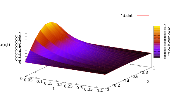

 . Therefore we will define only two arrays in order
to store the values
  and
and  at time
 .
.


 ,
,  and
and 
 in
three columns. When a time slice is printed, the program prints an empty line so
that the output is easily read by the three dimensional plotting function
  can be made with the
 for a fixed value of
  we first note that an
empty line in the file
  . We save the results in the file


 . We compute the relative error

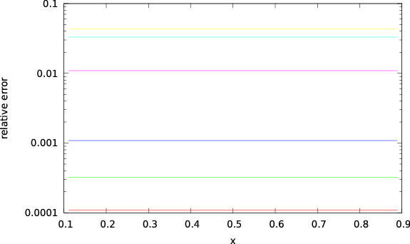


 for the diffusion, or random walk,
problem, we should impose the normalization condition (
 defined for
 ![x ∈ [0, 1]](main_latex3019x.png) the relation
becomes
the relation
becomes
![x ∈ [0,1 ]](main_latex3021x.png) , then the points
, then the points  and
and  are identified and we
obtain

 , we obtain
  ,
,
 .
.
 , we apply equation (
 ,
,  . In order to take into account the cyclic topology we
take


 is the point
  and the
neighbor to the left of the point
  is the point
  . For the rest of the points
 equation (
 , the boundary conditions (
 are chosen so that the particle is located at
 . For each instant of time we perform measurements in order to verify
the equations (
 const.
 and we should check that its value is
conserved and is always equal to 1.
 is a discrete estimator of
the expectation value of the distance squared from the initial position.
For small enough times it should follow the law given by equation (
 ,
,
 and
and  . The latter are measured in order to check if for large enough
times they obtain the
  const.

 for all
 ,
,


 ,
,  ,
,  .
.
 ,
,  ,
,  ,
,  ,
,  ,
,  are found in
columns 2, 3, 4, 5, 6 and 7 respectively of the file
  ,
,  ,
,
 ,
,  ,
,  ,
,  .
. 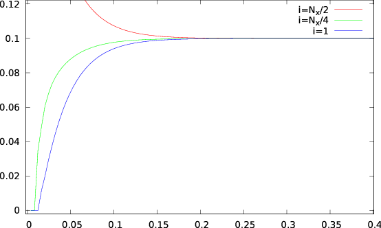


 can be easily confirmed by inspecting the values recorded
in the file
  can be confirmed with the commands
 with the commands
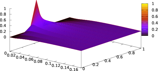


 in a thin rod satisfies equation
(
 . The initial temperature distribution at
  is given by
the function
![{ 0.5 x ∈ [x ,x ]
u(x,0) = 1 2 ,
0.3 x ∕∈ [x1,x2 ]](main_latex3095x.png)
 and
and  .
.
 for
for  ,
,
 ,
,  ,
,  . Take
  and
and  . Do the
same for
  by choosing appropriate
  and keeping
 . Plot the functions
  in the same plot.
 ,
,  ,
,  ,
,  ,
,  ,
,  ,
,  . Take
 and choose an appropriate value for the corresponding
 .
.
 .
. .
.
 in a thin rod satisfies the
equation

 , and when

![( [ (2πx)]
{ 0.5 1 − cos -b- 0 ≤ x < b
u(x,0) = 0 b ≤ x ≤ 1 .
(](main_latex3124x.png)
 for
for  ,
,
 and for
 ,
,  ,
,  , by taking
 ,
,  . Do the same for
  by choosing
appropriate
  . Plot the functions
  in the same plot.
 ,
,
 and
and  for
for  . Plot the functions
 in the same plot.
 for
for  and
and
 for
for  . Plot the functions
  in the
same plot. Comment on the effect of the parameter
  on your
results.
 in a thin rod of length
  satisfies
equation

 is the
  -dependent thermal diffusivity. The
temperature of the rod at its ends is such that
  , and at
time
  , the temperature distribution is

 ,
,  ,
,
 ,
,  ,
,  ,
,  and
and  interactively. On exit, the program
calculates
  and writes the points
  in two
columns to a file
  ,
,  ,
,  ,
,  ,
,  ,
,  and calculate
  for
for  . Plot the functions
 in the same plot.
 and
and  for
for
 . Plot the functions
  in the same plot.
 as a real
symmetric matrix in an appropriately chosen basis of the Hilbert space
  of
quantum mechanical states. The energy spectrum is obtained from the
eigenvalues of this matrix and the numerical problem reduces to that of
the diagonalization of a real symmetric matrix. Since the Hamiltonian is
represented in
  by an infinite size matrix, we have to restrict ourselves to a
finite dimensional subspace
  of dimension
  . In this space the
Hamiltonian is represented by an
  real symmetric matrix. The
eigenvalues of this matrix will be calculated numerically using standard
methods and the energy eigenvalues will be obtained in the
  limit.

 ,
,  so that
we can express the above equation using dimensionless terms:

 ,
,  and
and  ,
then we obtain

 ,
,  and
and  are now dimensionless. The operator
  can be
diagonalized with the help of the creation and annihilation operators
  and
and  ,
defined by the relations:

![[a, a†] = 1,](main_latex3201x.png)

 ,
,  of
of  span the Hilbert space of states
  and satisfy the relations


 is given by the wavefunctions:
 are the Hermite polynomials.


 in this representation are:
 can be calculated from equation (9.12) :

 from the matrix
product of
  with itself.
 .
.

 of the subspace
  of the Hilbert space
of states
  . We will restrict ourselves to states within this subspace and we will
use the
  dimensional representation matrices of
  ,
,  and
and  in
in  .
For example, when
  we obtain


 of
the
  matrix
  . Instead of reinventing the wheel, we will use ready
made routines that calculate eigenvalues and eigenvectors of matrices found in the
Lapack library. This library can be found in the high quality numerical software
repository
  .
The number of rows
 using the same matrix. The subroutine can be used in two ways:


 . The matrix
  of
of  and the coupling constant
  .
Then the program computes the eigenvalues
  of the
  matrix
  , which represents the action of the operator
  in the
 representation in
  . The tasks are allocated to the
subroutines
  matrix
  . First, the matrix
  is
calculated and then
  is obtained by computing its fourth power. The
matrix
  can also be calculated analytically and this is left as an
exercise to the reader. The subroutine
  using the result for
  given by
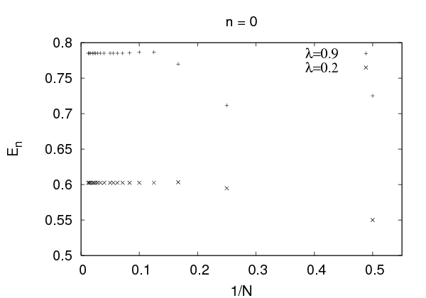


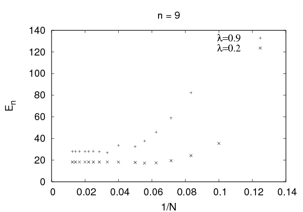


 and
and  . The
. The  choice leads us
to the simple harmonic oscillator and we obtain the expected solutions:
 ,
,  and the eigenstates (eigenvectors of
 )
)  . Similar results can be obtained for larger
 .
.
 , the finite
  calculation contains systematic errors
from neglecting all the matrix elements
  for
for  or
or  . Our
program calculates the eigenvalues
  of the finite matrix
  ,
,
 and one expects that


 -th level eigenvalue of the Hamiltonian
  . In practice the limit
 and
and  is calculated by computing
  numerically for
increasing values of
  . If convergence to a desired level of accuracy is achieved
for the accessible values of
  , then the approached limit is taken as an
approximation to
  . This process is shown graphically in figures
  . Convergence is satisfactory for quite small
  for
for  but
larger values of
  are needed for
  . Increasing the value of
  for fixed
 makes the use of larger values of
  necessary. Similarly for a given energy
level
  , increasing
  also makes the use of larger values of
  necessary. A
session that computes this limit for the ground level energy
  is shown
below
 convergence of
  and that we can take
  . For higher
accuracy, a computation using larger
  will be necessary.
 of an operator
 when the anharmonic oscillator is in a state
 :
:


 are the eigenvectors of the finite
  matrix
  computed numerically by
  , where

![cm (N, λ ) = H [n ][m ].](main_latex3328x.png)

 ,
,  and
and  . Taking into account that
 , we obtain the uncertainties


 and
and 
 . Their product
should satisfy
 . The results are
shown in table
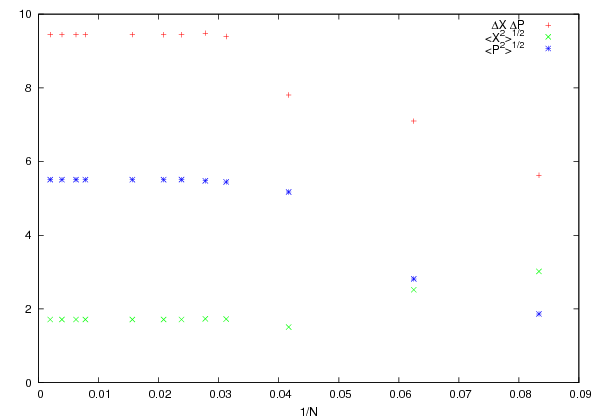


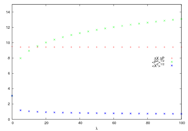


 limit. As shown in figure
  dominates in this limit
and the expectation value
  decreases. This means that states that
confine the oscillator to a smaller range of
  are favored. This, using the
uncertainty principle, implies that the typical momentum of the oscillator
also increases in magnitude. This is confirmed in figure
  to increase with
  . In order to
understand quantitatively these competing effects we will use a scaling
argument due to Symanzik. We redefine
  ,
,  in the
Hamiltonian
  and for large enough
  we
obtain
 is the Hamiltonian of the anharmonic “oscillator” with
 . Since the operator
  is independent of
  , the energy spectrum will
have the asymptotic behavior

 we have that

 . For large values of
  , the authors
obtain the asymptotic behavior


 . This relation is tested
in figure
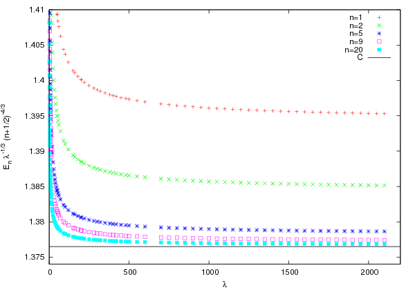


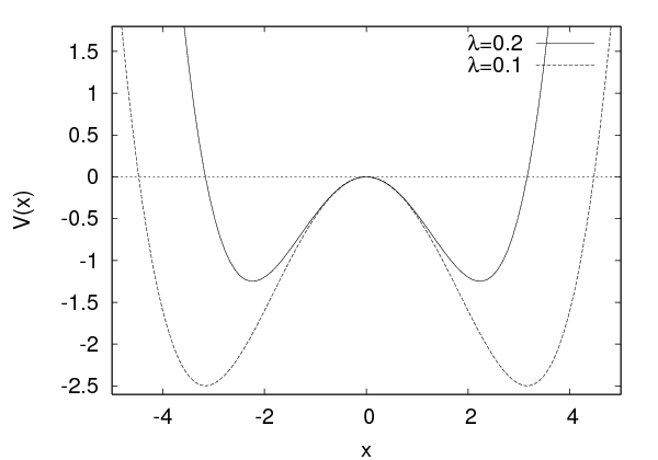


 , therefore


 and
and

 and
and  are localized to the left and right well of the
potential respectively (see also figure
  . The resulting
program can be found in the file
  and
and  ? The answer to this question is obtained from the study of the
expectation value of the position operator
  in each one of them. We know
that when the particle is in one of the energy eigenstates, then we have
that

 is even. Therefore

 and that the amplitudes
 .
Also
 . Therefore, if we have that
  and
and
 , we obtain

 , the subroutine
  in the columns of the matrix
 with the classical values
 as
as  is increased.
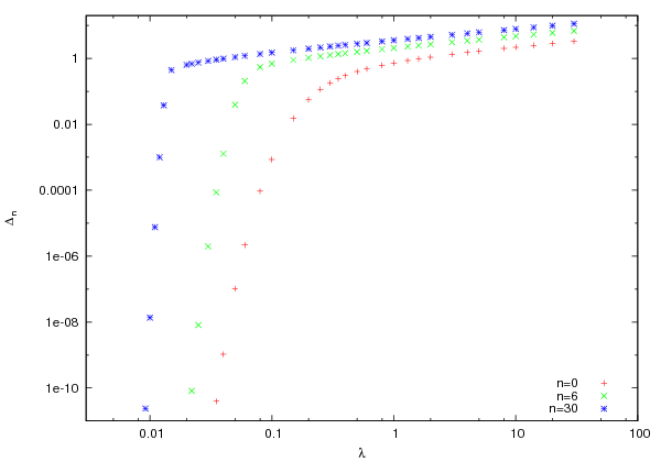


 for
for  analytically. Calculate its
eigenvalues for
  . Compare your results with the numerical values
that you obtain from your program.
 and that they form an orthonormal basis
  .
.
 and
and  for
for  with an accuracy better
than
  %.
%.
 can you calculate
  for
for  with an accuracy
better than
  % when
  ?
?
 and
and  for
for  with step
  by
achieving accuracy better than
  %. How large should
  be taken
in each case?
 in the
  representation analytically. Modify the program in
 by computing the exponent (cpu time)
 for
for  .
.
 and
and  . What is the largest value of
 that you can study given your computational resources?
 for
for
 and then fit your results to a function of the form
 . What is the accuracy in the calculation of
the coefficients
  ,
,  and
and  and how good is the agreement with
equation (
 ,
,  and the corresponding
products
  .
.  . Repeat your calculations for
  .
.
 .
.
 .
.

 for
for  ,
,  and
and  .
.
 ,
,  and the products
  .
Calculate the expectation values
  ,
,  and
and  for
for
 ,
,  and
and  .
.
 for
for  and
and  .
Calculate the difference
  and comment on your
results.

 of the previous problem with
 and
and  respectively. Explain your results.
 given by equation (
 with the
classical values
  for
for  .
.
 for
for  and
and  .
.
 ,
,  . Calculate these
quantities for the anharmonic oscillator and the double well potential for
 and
and  . What do you conclude from your
results?
 , without spin, moving in one
dimension, in a static potential
  . We will only study bound states. The
solutions in this case yield the discrete energy spectrum
  as well as
the corresponding eigenstates of the Hamiltonian
  in position
representation.
 , and one that can be applied to
more general cases. The first method is introduced only for educational
purposes and the reader may skip section
  , which are the position representation of the energy
eigenstates, satisfy the Schrödinger equation


 . Equation (
 such that
  . The numbers
  are real and they are the (bound) energy spectrum of the particle in the
potential
 . The minimum energy
  is called the ground state energy and
 . According to
the Heisenberg uncertainty principle, in this state the uncertainties in momentum
 and position
  so that
 form an orthonormal basis
 which represents the state
 is given by the linear combination


 are complex numbers
that give the probability
  to measure energy
  in the state
 .
.
 the function

 , i.e. the probability
of detecting the particle in the interval
 ![[x1,x2]](main_latex3560x.png) is given by
is given by

 axis).
 of this quantum mechanical system are
functions of the position and the momentum and their quantum mechanical
versions are given by operators
  . Their expectation values when the
system in a state
  are given by
 , the
function
  and the parameters so that we deal only with dimensionless
quantities. Equation (
 which is defined by the parameters of the
problem
 . We define
 and we obtain


 ,
,  and
change notation to
  ,
,  . We obtain


 and we
obtain

![[x, p] = iℏ](main_latex3593x.png) becomes
becomes ![[˜x, ˜p] = i](main_latex3594x.png) . The kinetic energy
. The kinetic energy
 is given by


 instead of
 .
.
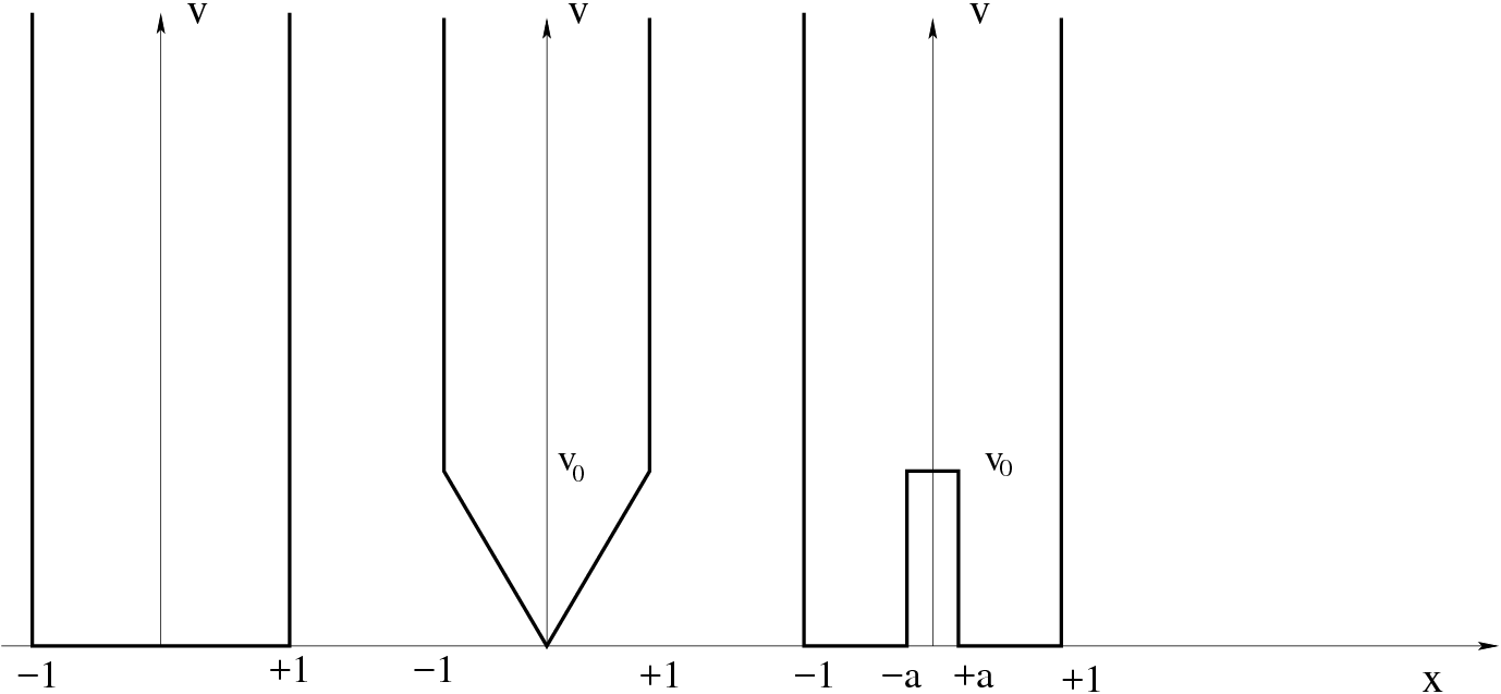
 where a particle is confined within the interval
![[− L∕2,L ∕2]](main_latex3602x.png) :
:

 and the dimensionless variable
  corresponds to
  when
when  is measured in length units.


 for
for  and one with odd parity

 for
for  .
.


 .
.


 depends on the normalization of the wave function. Therefore
we can set
  originally and then renormalize the wave function so
that equation (
 . The problem is that the energy
  is unknown. If the energy
is not allowed by the quantum theory we will find that the boundary
conditions

 .
. 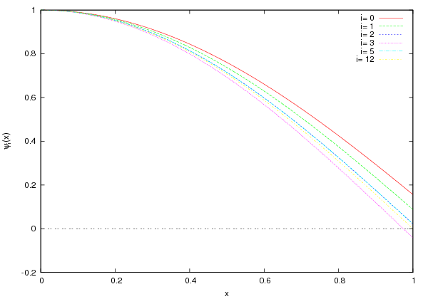


 that is lower than the
one we are looking for. We can use estimates from known solutions
of similar looking potential wells or simply start from a value slightly
higher than the absolute minimum of the potential.
 to
to  .
.
 and
we repeat.
 changes sign. Then we lower the energy by
 .
.
 for appropriately chosen
small
  .
. to
to  we use the 4th order
Runge-Kutta method


 and
and  respectively and
  . The file

 changes (
 ). Then the value of the energy is overestimated
and we change the sign of the step
  can be studied. The full program is listed
below:


 . The
convergence can be studied graphically in figure
  is excellent.


 are positive numbers. A qualitative plot of these
functions is shown in figure
  , whereas for the double well
potential
  and
and  .
. , the energy levels of all the potentials
that we studied above tend to have identical values. This happens because, when
the particle has energy much larger than
  , the details of the potential at the
bottom do not influence its dynamical properties very much. For the triangular
potential, the energy levels have higher values than the corresponding ones of the
square potential. This happens because, on the average, the potential energy is
higher and the potential tends to confine the particle to a smaller region (
 is
decreased, therefore
  is increased). This can be seen in figure
  and
and
 . The first one represents a state where
the particle is localized in the left well and the second one in the right.
This is shown in figure
  the two wells decouple and
the wave functions
  become equal to the energy eigenstate wave
functions of two particles in separate infinite square wells of width
  with energy eigenvalues
  . The difference of
  and
and  from these two values is due to the finite
  (see problem
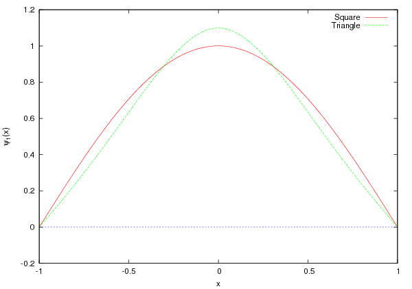
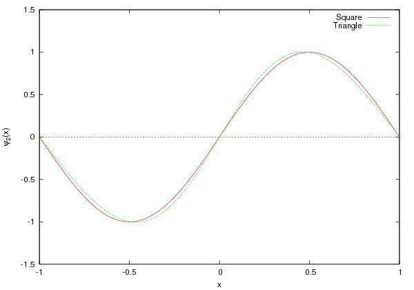

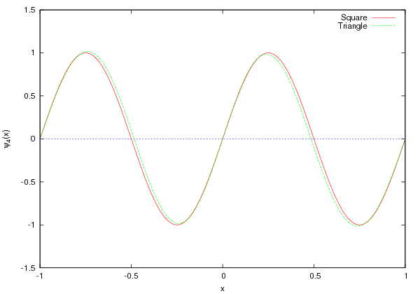
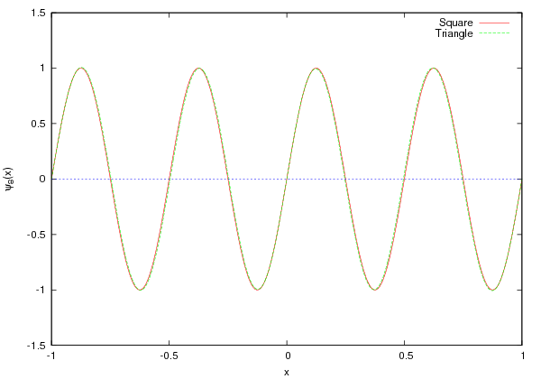
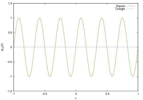


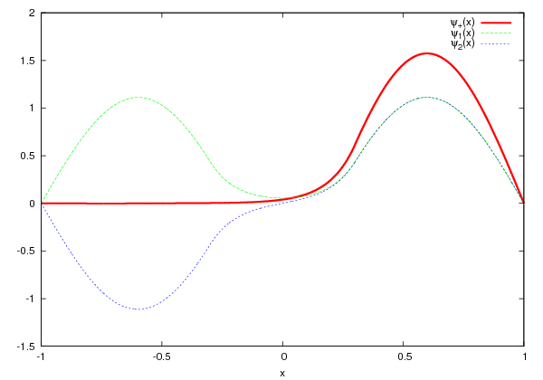
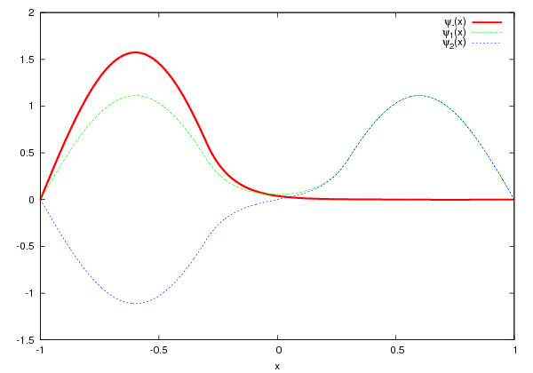
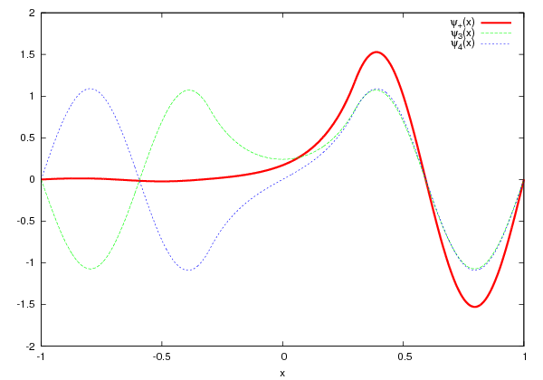
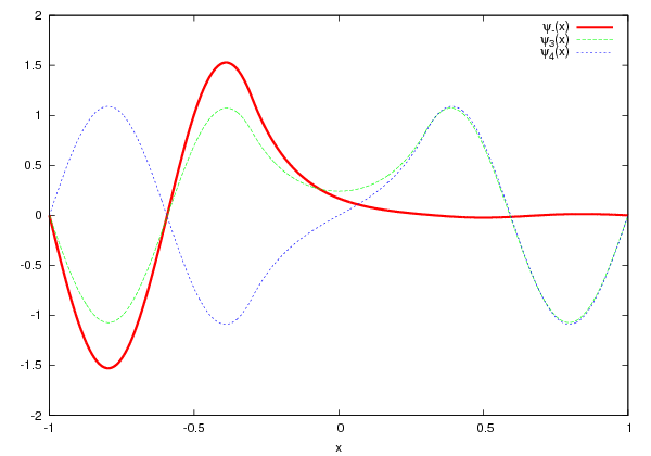
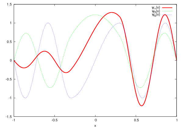
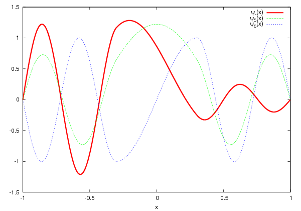


 . We used this
assumption in equations (
 , the wave function is almost zero around
  and
the integration from
  to
to  will be dominated by numerical
errors. The same is true when the particle has to go through high potential
barriers.


 , the
convergence of the algorithm becomes harder. You can understand this by
realizing that in the integration process the solution is evolved from the classically
allowed into the classically forbidden region so that an oscillating solution
changes into an exponentially damped one. But as
  there are two
solutions, one that is physically acceptable
  and one that is
diverging
  which is not acceptable due to (
 . For this reason it is preferable to integrate from the exponentially
damped region towards the oscillating region. The idea is to start integrating
from these regions and try to match the solutions and their derivatives at
appropriately chosen matching points. The matching is achieved at a
point
  by trying to determine the value of the energy that sets the
ratio

 within the classical region (
 ) and usually
we pick a turning point
 . By renormalizing
  we can
always set
  , therefore
  means that
 . The denominator of (
 ,
,  ,
,
 ,
,  . This choice depends on the potential
 . Usually we take
  ,
,  to
be zero or exponentially small (e.g.
  ,
,  ). The
corresponding values of the derivatives
  ,
,  are also taken to be small. The arbitrary normalization of
  allows
these initial values to be chosen in a crude way. The relative sign of
the derivatives at large
  (determined e.g. by the parity of the wave
function for even potentials) is also taken care by the renormalization
of
  when applying the matching condition. For an infinite well,
the points
  .
.
 and of the energy variation
step
  .
.
 . Choose the solution that is at the left most side
 ,
, .
.
 ,
, .
.
 , so that
 .
.
 of equation (
 for appropriately chosen
  , the calculation ends.
The result for the energy eigenvalue and eigenfunction is considered to
be determined with adequate accuracy and we may proceed with the
analysis of the results.
 changes sign it means that we have crossed the energy
eigenvalue. Reverse the direction of search by taking
  .
.
 and repeat by going back to the fourth
step.
 corresponding to the eigenvalue
  . We normalize the
wave function according to equation (
 of the wave function which is related to
  by
by  .
.
 is coded in the function
  ,
,
 ,
,  ,
,  to the calling program. These functions are put in a separate file for each
potential that we want to study. The name of the file is related to the form
of the potential, e.g. we choose

 ,
,  . The energy of
the ground state is found to be
  . The wave
function is stored in the file
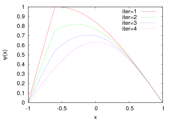
 on a state
  can be easily calculated in the
position representation by its action on the corresponding wave function
  .
The action of the operators


 of the
operator
  when the system is at the state
  . Interesting examples are the
observables “position”
  , “position squared”
  , “momentum”
  , “momentum
squared”
  , “kinetic energy”
  , “potential energy”
  , “energy” or
“Hamiltonian”
  whose expectation values are given by the relations
 as well as
equations (10.15) and (10.16) . Especially interesting are the “uncertainties”
 ,
,  that satisfy the inequality (“Heisenberg’s
uncertainty relation”)

 , we obtain that
 . Other operators need a numerical approximation
for the calculation of their expectation values. If the values of the wave
function are given at
  equally spaced points
  , then we
obtain
 and
and

 . Special care should be taken at
the endpoints of the interval
 ![[x ,x ]
1 N](main_latex3811x.png) . As a first approach we will use the naive
approximations
. As a first approach we will use the naive
approximations

 ,
,  ,
,  ,
,  ,
,  ,
,  can be
found in the file
  in
the format produced by the program in
  pairs. It is not necessary to have the wave
function properly normalized, the program will take care of it. If this data is
stored in a file
  , the value of the
energy
 ,
,  ,
,  ,
,  ,
,  ,
,  and
and  to the
  . In this section we will revisit the problem by using the
position representation. We will calculate the eigenfunctions
  that
diagonalize the Hamiltonian (
 in equation (
 . For
. For  we obtain the harmonic oscillator with

 are the Hermite polynomials.
 ,
,  . You are encouraged to test the
influence of other choices on the results.
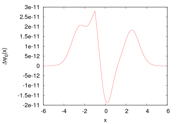


 –
– . The values of the energy
 for
for  are in agreement with (
 .
.
 ,
,  ,
,  ,
,  ,
,  and
and
 . These are easily calculated using equations (
 ,
,  ,
whereas

 with accuracy
  and
and
 with accuracy
  . The expectation values
  ,
,  are shown
in table


 . We copy the file
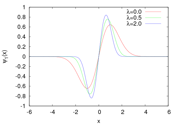
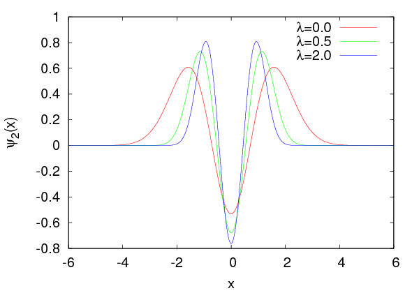
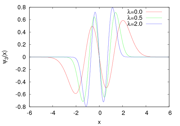
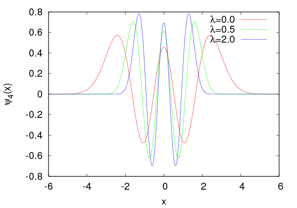
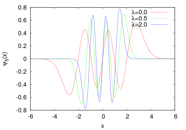


 the
particle becomes more confined in space as expected. In table
  for
for  . By increasing
  ,
,  is increased.
Table
  ,
,  and
and  for the
anharmonic oscillator for the states
  ,
,  . By increasing
  ,
,
 is decreased and
  is increased. The product of the
uncertainties
  seems to be quite close to the corresponding values for the
harmonic oscillator. The results should be compared with the ones obtained in
table
 in (
in ( . Equation (
 are related to the energy values
  by
by

 . The minimum is
located at
  and its value is
  . The code for this
potential is in the file


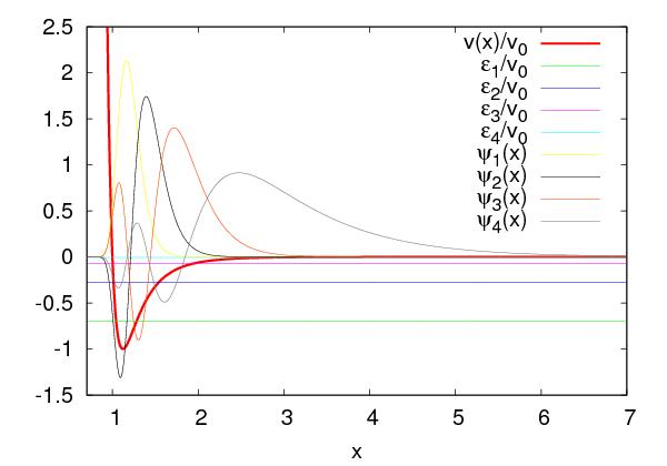


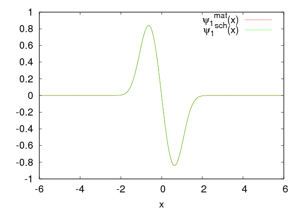
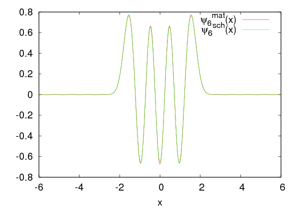

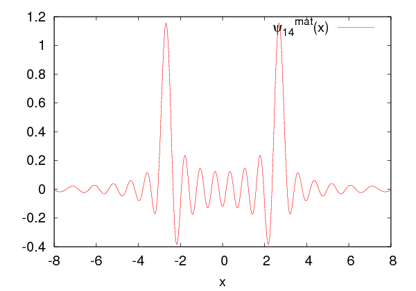


 and
and 
 .
The results are plotted in figure
  within the attained accuracy as expected for real, bound
states
 can be computed using the Simpson rule

![[a,b]](main_latex3966x.png) is discretized by
is discretized by  points
  where
where  is even. Each interval
 ![[x ,x ]
i i+1](main_latex3970x.png) has width
has width  .
.
 of the calculated wave function
 .
.
 . This is the problem of the (finite) potential well.
Solve the problem for
  and
and  . How many bound states do
you find? Next study the influence of the wall on the solutions. Introduce a
parameter
  so that
  and study the dependence of the
solutions on
  . Take
  and
compute the difference of the first two energy eigenvalues. Estimate the
accuracy of the method. Next lower the value of
  until there is no
bound state. What is the relation between
  and
and  when this happens?
Compare with the analytic result which you know from your quantum
mechanics course.
  , take
  to the double well potential. Observe the (almost)
degenerate states and plot the wave functions
  ,
where
  is odd. Compare the results with the corresponding energy levels
and eigenfunctions of the infinite square well. Increase
  to the point
where you cannot solve the problem numerically.
  the numerical effort is increased. For
  the wave
function is almost zero and it is hard to obtain the non trivial wave function
for
  . As the accuracy deteriorates, you should increase

 and
and

 and
and

 . In each case
calculate
  ,
,  ,
,  ,
,  ,
,  ,
,  ,
,  .
.
![[x1,x2]](main_latex4005x.png) given the wave function calculated
by the program in the file
given the wave function calculated
by the program in the file ![[− x1,x1]](main_latex4006x.png) where the probability to find the particle inside them is equal to
where the probability to find the particle inside them is equal to
 .
.
 ,
,  ,
,  ,
,  ,
,
 ,
,  ,
,  and plot each expectation value as a function of
 .
.


 for which
  . Calculate the
energy levels
  of the bound states numerically by setting
  in
equation (
 . Plot the potential
  and the
corresponding eigenfunctions. Calculate the expectation values of the
position and momentum, the uncertainties in position and momentum and
their product. Repeat for
  .
.

 is real. Calculate
  for the harmonic
oscillator for
  and show (numerically) that
  .
.

 ,
,
 ,
,  ,
,  and obtain


 ,
,  , and
, and
 is a Laguerre polynomial given by


 . You can take
  ,
,  and calculate
  ,
,  ,
,
 ,
,  ,
,  ,
,  ,
,  .
.
 and
and  . Calculate the
wavefunctions using the program
  and compare the two results.

![N∑−1
|n ⟩λ = H [n][m ]|m ⟩
m=0](main_latex4062x.png)
 ,
,  . From
  and
and  for
for  and determine the accuracy achieved by the calculation
for each
  . For which values of
  do you obtain large discrepancies
between your results? Remember that for large
  , the states of high energy
contribute more than for small
  . Figure
  does not apply. Second, the geometry of
the path of the random walker has fractal dimension which is larger than
one
 from which the next one
  is generated by
the relation
 ,
,  and
and  . In the bibliography, there is a
lot of discussion on the good and bad choices of
  ,
,  and
and  , which
depend on the programming language and whether we are on a 32–bit
or 64–bit systems. For details see the chapter on random numbers in
 determines the maximum period
 steps, then
the exact same sequence will be produced and
  will be the period of the
sequence. Since there are at most
  different numbers, the period is at most
equal to
  . For a bad choice of
  ,
,  and
and  the period will be much smaller.
But
  cannot be arbitrarily large since there is a maximum number of bits that
computers use for the storage of integers. For 4-byte (32 bit) unsigned integers the
maximum number is
  , whereas for signed integers
  . One can
prove
 ,
,  and
and  results in a sequence which is a permutation
 of the numbers
  . This is good enough for simple
applications that require fast random number generation but for serious
calculations one has to carefully balance efficiency with quality. Good quality
random generators are more complicated algorithms and their states are
determined by more than one integer. If you need the source code for such
generators you may look in the bibliography, like in e.g.
  ,
,  and
and  :
: ,
,  and
and  . This is the choice of
Lewis, Goodman and Miller (1969) and provides a generator that passes
many tests and, more importantly, it has been used countless of times
successfully. One technical problem is that, when we multiply
  by
by  ,
we may obtain a number which is outside the range of 4-byte integers
and this will result in an “integer overflow”. In order
 positive, 32-bit (4 byte), signed integers. Schrage has proposed to use the
relation
positive, 32-bit (4 byte), signed integers. Schrage has proposed to use the
relation![( [ ]
||{ a (xi− 1 modq ) − r xi−q1- if it is ≥ 0
[ xi−1]
(axi−1) modm = || a (xi− 1 modq ) − r -q-- + m if it is < 0
(](main_latex4108x.png)
 ,
, ![q = [m ∕a ]](main_latex4110x.png) and
and  . One can show that if
 and if
  , then
  ,
,
![0 ≤ r[x ∕q] ≤ m − 1
i−1](main_latex4115x.png) and that (
and that ( . The proof of the above statements is left as an exercise to the
reader.
 which appears once in the sequence. This
adds a
  % overhead, depending on the compiler. If you don’t
care about that, you may remove the line. Note that the number
  , where
 , which are subsequently mapped on
the plane. This is done by taking the integer part of the numbers
  with
with  and
and  is the random number produced by the
generator:
 points used in the plots in figures
  that it produces, do not pass the
  test when we have more
than
  points, which is much less than the period of the generator. In order to
avoid such problems, there are many solutions that have been proposed and the
simplest among them “shuffle” the results so that the low order serial
correlations vanish. Such generators will be discussed in the next section.
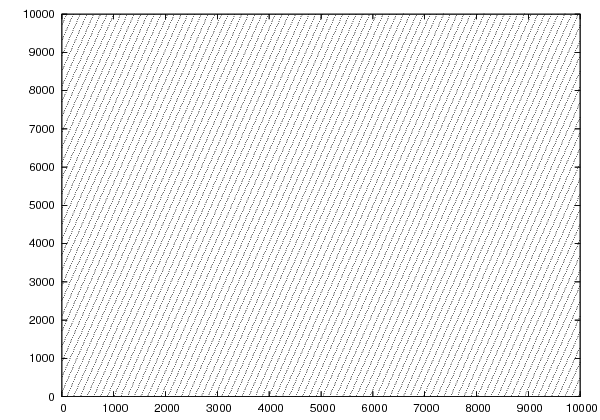
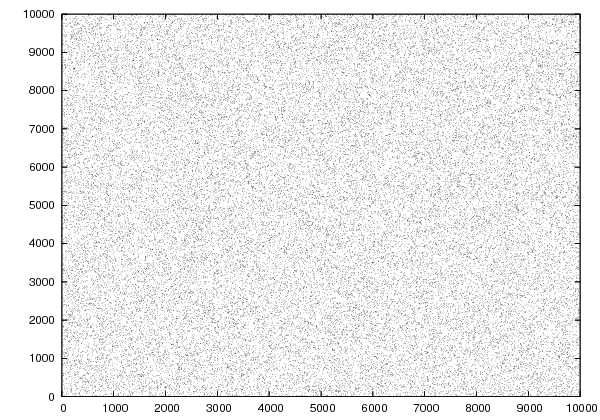
 . The reciprocal of the number following the option
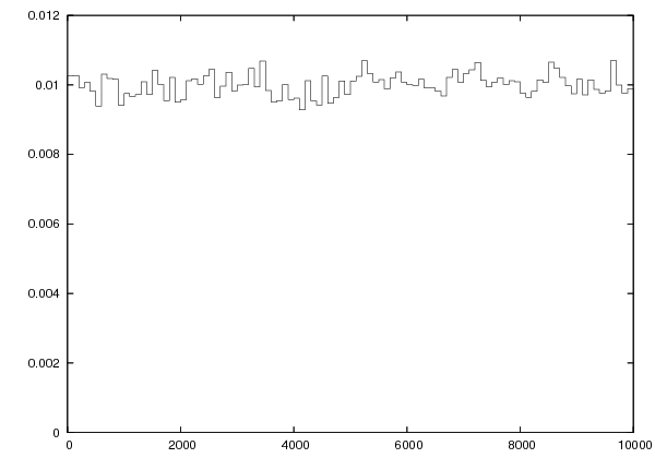

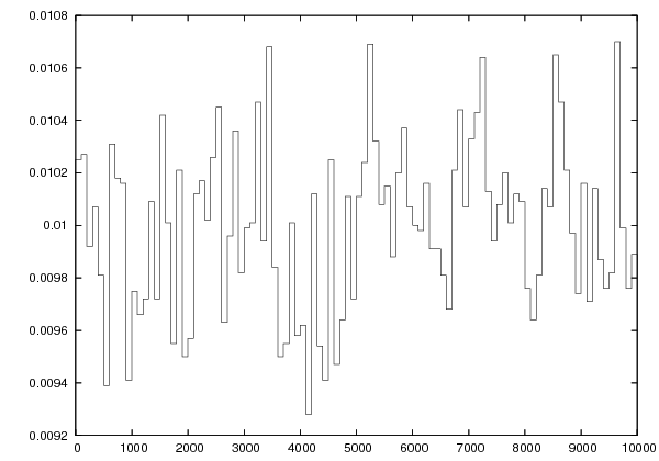
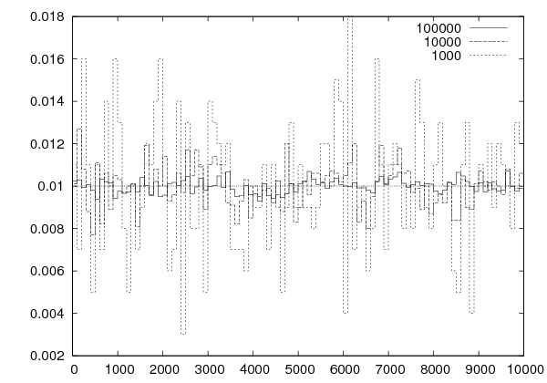


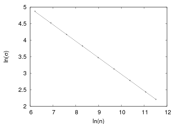

 of the sample, we calculate the standard
deviation
 is the sequence of random numbers. Figure

 we can use a sequence of uniformly distributed random
numbers in the interval
  as follows: Consider the cumulative distribution
function
 in the interval
 ![(− ∞, x]](main_latex4142x.png) and it
is equal to the probability
and it
is equal to the probability  . If
. If  is uniformly distributed in the
interval
  then we have that
  . Therefore
  is such
that
  and follows the
  distribution. Therefore, if
 form a sequence of uniformly distributed random numbers, then the
numbers

 .
.


 is the error function. The error function, as
well as its inverse, can be calculated numerically, but this would result in a slow
computation. A trick to make a more efficient calculation is to consider the
probability density
  of
of  and
and 

 ,
,  . Then we have that


 of uniformly distributed
random numbers and take
 , which follow the
Gaussian distribution
 is listed below:


 (this is what the “flag”
  and others.
 (
( included,
  excluded) of the type
  . Moreover, it passes all known statistical tests for statistically
independent sequences of random numbers and it is very cleverly and efficiently
implemented. It generates sequences of random numbers by using a relation of the
form

 . The matrix
  has integer entries and has special
properties. The trajectories of the above map have very strong chaotic
behavior and this is the reason for the high quality of the produced random
numbers
 , the computational cost per random number
using (

 and standard deviation
  of the distribution by changing the values of the
variables
  . The minimum distance between
the lattice sites is
  (lattice constant). The vector that describes the change of
the position of the particle during the
  -th jump is a random variable
  and it
always has the same magnitude
  . This means that, given the
position
  of the particle at time
  , its position
  at time
 is
is


 and
and  are uncorrelated for
  and we have that

 are equally probable, therefore we obtain

 occur with the same frequency and they cancel each other.
Therefore
  for
for  . Since the magnitude of the vectors
  is
constant, we obtain

 of length
  to occur
is
 is the number of nearest neighbors of a lattice site. This
probability depends on the length of the path and not on its geometry.
This can be easily seen using the obvious relation
  ,
since there are exactly
  equally probable cases. The partition function
is

 .
.
 the particle is displaced from its original position
by


 .
.


 means asymptotic behavior in the limit
  . For a classical
walker
  , whereas for the random walker
  .
.
 with equal probability.
The SAW is a NRRW with the additional requirement that, when the
walker ends in a previously visited position, the ... walking ends! Some
models studied in the literature include, besides the infinite repulsive force,
an attractive contribution to the total energy for every pair of points of
the path that are nearest neighbors. In this case, each path is weighted
with the corresponding Boltzmann weight according to equation (
 .
Even though the paths differ microscopically, their long distance properties are
the same. They are examples of models belonging to the same
 such that for
  we have similar behavior
given by equation (
 the attractive interaction
dominates, the paths collapse and we obtain
  . For
. For  we
have that
  . For more information we refer the reader to the book of Binder
and Heermann
  ,
,  , etc
, etc
 is written to
 of the points visited by the walker in
each path is written to
  is chosen and it
is added in the current position
  . The choice on
  is made in
the line
 because the function
  . We use the construct
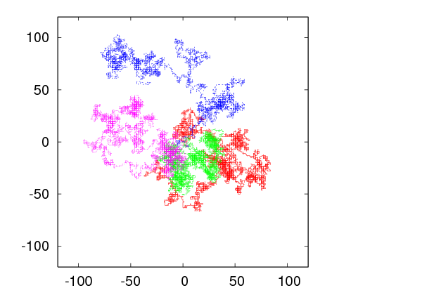

 for
for  which confirm equation
(
 .
. 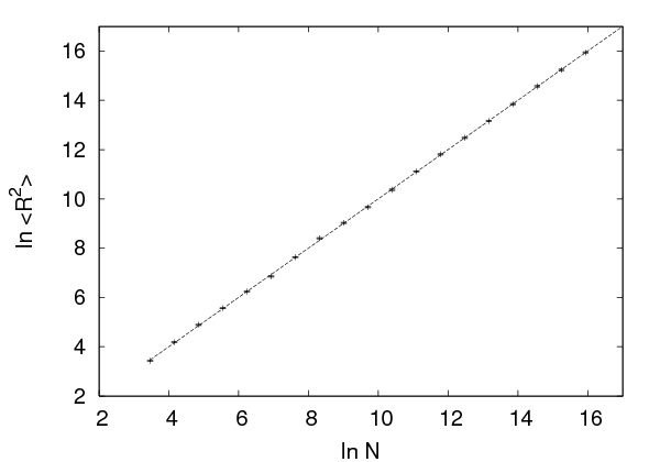


 in the first column and with
  in the second. The
command
 going through the points (
 ,
, ). You can also use the
  , where
  is the number of measurements. For the same
reason
 . Construct the plot
of relative frequencies together with the plot of the probability density
function.
 . Construct the plot of relative
frequencies together with the plot of the probability density function.
 random numbers using the function
  then
then
 and we obtain a linear relation between displacement–length of
path. The quantity
  is the expectation value of the speed of the particle.
Compute
  for large values of
  .
.
 and the rest equal
to
  . Compute the expectation values
  and
and  and use them
to calculate the average speed of the particle. Check the validity of the
relations
  and
and 
 . What is the
relation between
  ,
,  and
and  ?
?
 , she should run the command
  . Calculate
  and
and  numerically for
  . Are they really equal to zero? Why? How
does this depend on the number of measurements?
 . What happens as
  ?
Why?
 .
.
 can
you simulate? Check whether the CPU time for computing a given number
of random walks increases exponentially with
  . Search the internet
for the most efficient algorithm that simulates the SAW for large
 .
. . For simple macroscopic systems
  –
–  . For such
systems, it is practically impossible to solve the microscopic equations that
govern their dynamics. Even if we could, the solution would have had much
more information than we need (and capable of analyzing!). It is enough,
however, to know a small number of bulk properties of the system in
order to have a useful description of it. E.g. it is enough to know the
internal energy and magnetization of a magnet or the energy and density of
a fluid instead of the detailed knowledge of the position, momentum,
energy and angular momentum of each particle they are made of. These
quantities provide a thermodynamic description of a system. Statistical
physics makes an attempt to derive these quantities from the microscopic
degrees of freedom and their dynamics given by the Hamiltonian of the
system.
 . The energy spectrum of those states is assumed to consist of discrete
values
 . This system is in contact and interacts with a large
heat reservoir
 .
. which give the probability to find
the system in a state
  at time
  . These weights are the connection between the
microscopic and statistical description of the system. When this system is in
thermal equilibrium with the reservoir, its statistical properties are described by
the, so called,
  be the transition rates
  , i.e.

 is
is 
 is equal to
the rate that the system comes into the state
  from
from  , minus the rate of leaving the state
  . The second equation is a
result of the probability interpretation of the weights
  and states
that the probability of finding the system in any state is equal to 1 at all
times.
 are assumed to be time independent
and then the above system of equations for
  is linear with real
parameters. This, together with the constraint
  , implies
that
 and the system reaches equilibrium. Then, the
 converge to finite numbers
  . These are the equilibrium occupation
probabilities
 ,
with
  , the probabilities
  follow the Boltzmann distribution (Gibbs
1902)

 will be frequently
referred to as simply “the temperature” of the system, although, strictly speaking,
it is the inverse of it. Its appearance in the exponential in equation (
 is simply a conversion constant between units of
energy
 in equation (
 implies

 , one is interested only in the average value of such a quantity. This
is because the probability of measuring the quantity to take a value significantly
different from its average is ridiculously small. The average, or
 whose value in a state
  is
is  is equal
to

 for a typical thermodynamic
system is such that

 from its expectation value
 can be neglected. The limit
  is the so called
  of the
system

 of a thermodynamic system is defined by
 is the

 the free energy becomes the ground state
energy
 only the lowest energy term in equation (12.11) survives.
For this reason, equation (12.10) gives
  , which is the third law of
thermodynamics.

 to the microscopic degrees of freedom can be
derived from equations (


 Equation (
 . In such a case,
  counts,
more or less, the number of states of the system with energy close to
 .
.
 is
is .
Then the probability
  to measure energy
  in the canonical ensemble
is

 , we obtain


 is the number of degrees of freedom of the system and
  is a constant.
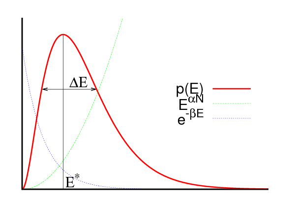


 and the deviation
  is a measure of the energy
fluctuations. The ratio
  drops with
  as
as  . Indeed, the
function


 decreases),
  shifts to larger values.
  is
proportional to the system size. By Taylor expanding around
  we obtain

 . Therefore


 has more than one equally probable
maxima
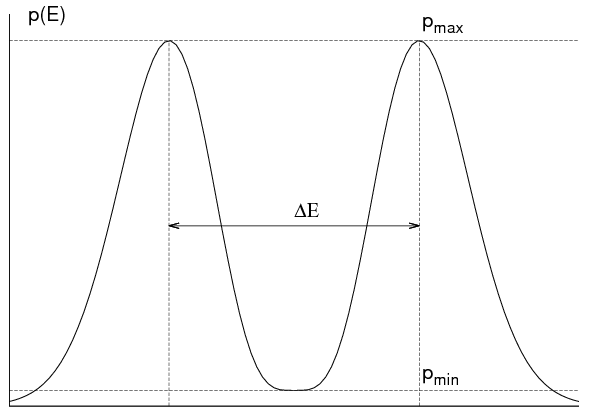


 is given by a distribution function
 which can be derived from the Boltzmann distribution (
 and
all its higher order moments, i.e. the expectation values
 . The most commonly studied moment is the second moment
(
 )
)

 is a measure of the fluctuations
of
  away from its expectation value
  . When
  we obtain


 , this role is played by
  ). For a magnetic system in a
constant magnetic field
  , such a quantity is the magnetization
 . If
. If  is
the magnetization of the system in the sate
  and we assume that its direction is
parallel to the direction of the magnetic field
  , then the Hamiltonian of the
system is


 in the
Hamiltonian. The quantities
  and
and  are called conjugate
 /
/ ) in a gas
or the chemical potential/number of particles (
 /
/ ) in the grand canonical
ensemble.


 is defined by the equation

 . Then the magnetic field
  is a function of the position
  and
interacts with the spin
  so that


 is
is


 and
and  are strongly correlated, i.e. they “vary together”
in the random samples that we take, the function (
 and
and  are not at all correlated with
each other, the terms
  in the sum over
  in the
expectation value
  cancel each other and
  is
zero
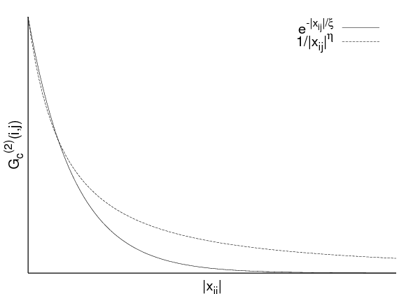


 takes its maximum value
  for
for  .
Then it falls off quite fast. For a generic system

 is the distance between the points
  and
and  . The
. The  , is a characteristic length scale of the system which is a measure of the
distance where there is a measurable correlation between the magnetic moments
of two lattice sites. It depends on the parameters that define the system
 . It is important to stress that it is a length scale that arises
 or the lattice
constant
  are parameters of the system which don’t depend on the dynamics. In
most of the cases,
  is of the order of a few lattice constants
  and such a
system does not exhibit correlations at macroscopic scales (i.e. of the order of
 ).
).
 . This can happen by fine tuning the parameters
on which
  depends on to their
  falls
off like a power (see figure
 is the number of dimensions of space and
  a
a  . Then the system is not sensitive to the
short distance details of the lattice and its dynamics are very well approximated
by continuum space dynamics. Then we say that we obtain the
  ,
,

 of a statistical system in the canonical
ensemble approximately. For this reason we construct a sample
 states


 which are distributed according to a chosen
probability distribution
  . We define the
  of
of  to
be
to
be

 , and we expect that

 so that the convergence of (
 , and equation (
 in a generic model. According to equation (
 is the probability of measuring energy
  in the system. A
qualitative plot of
  is shown in figure
  and
and  , therefore for
  and
and  the
qualitative behavior of the respective
  distributions is shown in figure
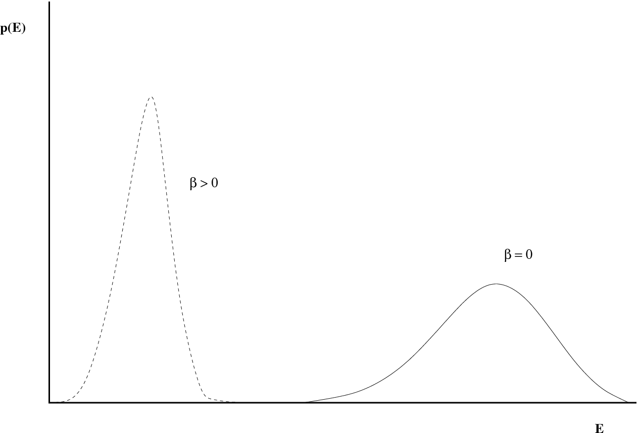


 in equation (
 const. in this
case
 we
have to obtain a good sample in the region where the product
  is
relatively important. The probability of obtaining a state such that
  is
non negligible is very small when we use the
  distribution. This can be
seen pictorially in figure
  .
.
 . If we choose a sample with probability


 and
the calculation of the expectation values (
 . This extra effort, however, is much smaller than the one required in order to
overcome the overlap problem discussed in the previous subsection.
 is not possible in a
direct way. For example, if we attempt to construct a sample according to
 by picking a state
  by chance and add it to the sample with
probability
  , then we have a very small probability to accept that state in the
sample. Therefore, the difficulty of constructing the sample runs into the same
overlap problem as in the case of simple sampling. For this reason we construct a
 , puts the system in a new state
  in such a way that it
has the
 from the
state
  to a new state
  satisfy the following requirements:
 and
and  and not on the path that the
system has followed on order to get to the sate
  (memorylessness)

 , i.e. the system has a
nonzero probability to remain in the same state
 the sample
  follows the
  distribution.
 . We may imagine that
this construction happens in “time”
  . In a Monte Carlo
 so that the convergence 4. is
fast.
 can become a non trivial task. If it turns out
not to be a typical state of the sample, then it could take a long “time” for the
system to “equilibrate”, i.e. for the Markov process to start sampling
states typical of the simulated temperature. The required time for this to
happen is called the
  and/or
 .
.
 it is possible to
reach any other state
  in a finite number of steps. If this criterion is
not satisfied and a significant part of phase space is not sampled, then
sampling will fail. Usually, given a state
  , the reachable states
  at
the next step (i.e. the states for which
  ) are very few.
Therefore the ergodicity of the algorithm considered must be checked
carefully
 distribution, the transition probabilities should be such that

 is equal to the
rate in which it leaves
  . From equation (

 after sufficiently long thermalization time.
By summing both sides of (
 that satisfy condition (
 and calculate the estimators
  from equation (
 has been
achieved.


 and
and

 for any other state
  . In order for (
 has to be chosen so that

 in two independent parts

 is the
  when the
system is in the state
  . Therefore the first step in the algorithm is to select a
state
  with probability
  .
.
 . If the
answer is no, then the system remains in the state
  . This way equation
(
 are called the
 and that the states
  are as much as
possible statistically independent from the original state
  . An ideal situation is
to have
  for all
  for which
  . As we will see in a
following chapter, this is what happens in the case of the Wolff cluster
algorithm.
 Ising Model


 . The geometry is determined by the distance of the
nearest neighbors, the
  , and the number of sites
  .
Each side consists of
  sites so that
  , where
  is
the dimension of space. The topology is determined by the way sites are
connected with each other via links. Special care is given to the sites
located on the sides of the lattice. We usually take
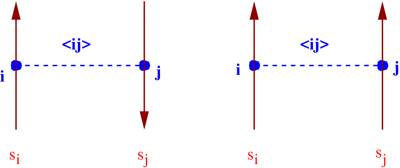


 or
or  . For the ferromagnetic model, each link
is a “bond” whose energy is higher when the spins on each side of the
link are pointing in the same direction and lower when they point in the
opposite
 whose direction is parallel to the direction of the
spins.
 lattice sites (or
  . The lattice has
  links (or
  , where
  is the pair of vertices on each side of the
link. We identify the sides of the square like in figure
 . The Hamiltonian of the system is given
by
 the system is
ferromagnetic.
 case. A link connecting
same spins has energy
  , whereas a link connecting opposite spins
has energy
  . The difference of the energy between the two states
is
  and the spin-spin dynamics favor links connecting same spins.
The minimum energy
  is
is . This is equal to

![∑ ∑ ∑ −βH [{si}] ∑ βJ∑ ⟨ij⟩sisj+βB ∑i si
Z = ... e ≡ e ,
s1= ±1s2=±1 sN= ±1 {si}](main_latex4684x.png)
 is a spin configuration of the system
 , which is equal to
  , i.e.
it increases exponentially with
  . For a humble
  lattice we have
 terms.
 has the interesting property that,
for
  , where
 ) and a
  ). The magnetization
  distinguishes between the two phases and it is called the
  is the Curie temperature
 , but it is non
analytic
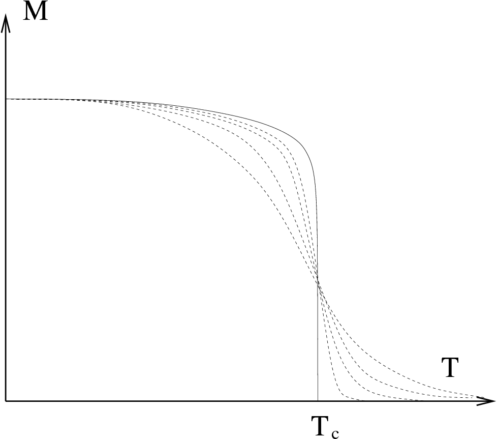
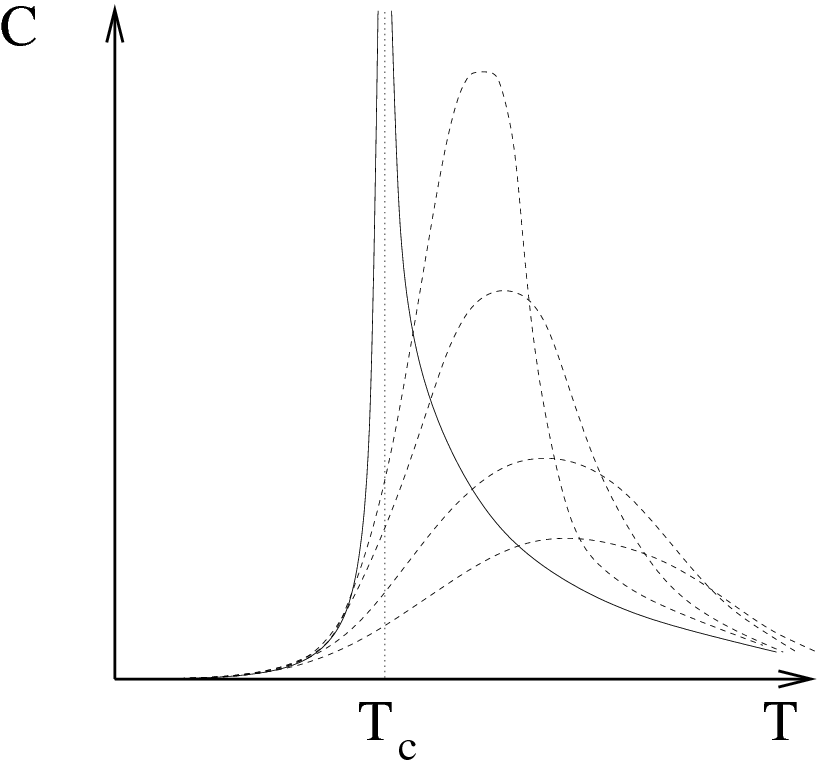


 the correlation function (
 . The correlation
length

 , the magnetization
 and the magnetic susceptibility
  according to the relations
 and nonzero magnetic field
  behaves
like


 model. The partition function (
 limit, where the finite
  analytic functions converge to a non analytic one. The loss of analyticity is
related to the appearance of long distance correlations between the spins
and the scaling of the correlation length according to equation (
 symmetry
represented by the transformation
  . The magnetization is zero in the
disordered, high temperature phase and non zero in the ordered, low temperature
phase. This implies that the magnetization is a non analytic function of the
temperature
 limit. In our case, this
occurs by tuning only one parameter, the temperature, to its critical value. A
unique, dynamical, length scale emerges from the correlation function, the
correlation length
  . Scale invariance
 when
when  . In the
critical region, all quantities which are functions of the distance become functions
only of the ratio
  . Everything depends on the long wavelength fluctuations
required by the symmetry of the order parameter and all models in the same
universality class have the same long distance behavior. This way one
can study only the simplest model within a universality class in order to
deduce the large distance/long wavelength properties of all systems in the
class.
 sites on each side so that
  is
the number of lattice sites (vertices) and
  is the number of links (bonds)
between the sites. The relation
  holds because we choose helical
boundary conditions as shown in figure
  we have one degree of
freedom, the “spin”
  which takes on two values
  . We consider the
case of zero magnetic field
  , therefore the Hamiltonian is given
by
 is a sum over the
  , corresponding to the pairs of sites
 . Then
  since each bond is counted twice in the
second sum. The partition function is
 ![∑ ∑ ∑ ∑ ∑
Z = ... e−βH[{si}] ≡ eβ ⟨ij⟩sisj.
s1=±1 s2= ±1 sN=±1 {si}](main_latex4739x.png)
 . According to (
 is
is

 is the
  when the system is in
the state
  and
and  is the
 . In order that the system changes states often enough, the
probabilities
  should be of order one and the differences in the
energy
  should not be too large. This means that the product of
the temperature with the energy difference should be a number of order
one or less. One way to accomplish this is to consider states that differ
by the value of the spin on only one site
  . Since the
energy (
 nearest neighbors, the change of the spin on
site
  results in a change of sign for
  terms
terms  in (
in ( . If the state
  is given by
 and the state
  by
by  (i.e. all the spins
are the same except the spin
  which changes sign), the energy difference will
be

 is randomly chosen then


 .
Remember that we should have
  and
and  . Therefore


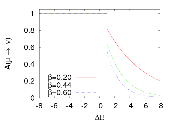


 on the change in energy for
different values of
  . We observe that this probability is small even
for zero energy change and we expect this method not to perform very
well.

 which are defined on
  lattice
sites. The most important part in designing the data structure in a lattice
simulation is to define the neighboring relations among the lattice sites
in the computer memory and this includes the implementation of the
boundary conditions. A bad choice of boundary conditions will make
the effect of the boundary on the results to be large and increase the
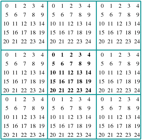

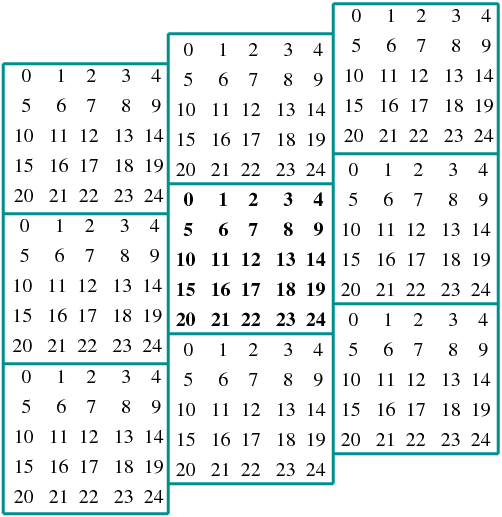

 ,
,  . Each spin is stored in an array


 to
to  .
This is shown in figures
  , where
  , as shown in figures


 when necessary. Therefore in a program that we want to
calculate the four nearest neighbors
  - all spins aligned) or a “hot” (
 - all
spins are equal to
  with equal probability
  ) initial configuration.
For large lattices, it is desirable to start in one of these states and then
lower/increase the temperature in small steps. Each time that the temperature is
changed, the spin configuration is saved and used in the next simulation.
  and consider the
transition to a new state
  which differs only by the
value of the spin
  (spin flip), whereas all the other spins are the
same:
 . The energy difference between the two states is
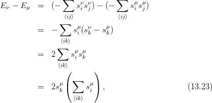
 , which you can prove
easily by examining the cases
  separately. The important property of
this relation is that it is local since it depends only on the nearest neighbors. The
calculation of the energy difference
  is fast and is always a number of order
one
 . If the energy decreases, i.e.
  , the new state
  is
accepted and “we flip the spin”. If the energy increases, i.e.
  , then
the acceptance ratio is
  . In order to accept the new
state with this probability we pick a random number uniformly distributed in
 . The probability that this number is
  is equal
to
 . Therefore if
  the change is accepted. If
 the change is rejected and the system remains in the same state
 .
.
 and these are the only values that enter in the
calculation of
  . Moreover, only the values that increase the energy, i.e.
 are of interest to us. Therefore we only need two values of
  , which
depend only on the temperature. These can by calculated once and for all in
the initialization phase of the program, stored in an array and avoid the
repeated calculation of the exponential
  which is expensive.


 has a
has a  symmetry because it is symmetric under reflection
of all the spins. The probability of appearance of a state depends only
on the value of
  , therefore two configurations with opposite spin are
equally probable. But such configurations have opposite magnetization,
therefore the average magnetization
  will be zero due to this
cancellation
 and its nearest neighbors. The energy
difference is already calculated by (
 , then the calculation of the magnetization
using the first method requires
  additions per
  Monte Carlo steps,
whereas the second one requires
  additions per measurement.
 , where
  for
the ground state in which all
  links have energy equal to
  . The
magnetization per site is

 , where
  for
for  (perfect disorder) and
 for the ground state at
  (perfect order). We call
  the
order parameter since its value determines the phase that the system is
in.


 independent
measurements the statistical error drops as
  . The problem of
determining how often we have independent measurements is very important and
it will be discussed in detail later in this chapter.
 is a constant parameter, whereas the arrays and variables
encoding the spins and the simulation parameters are put in the global scope. For
that, they must be declared as
  . The variable
  and the array
  according to the discussion on page
  and
and  direction and
  direction.


 . Those probabilities are going to be
used when
  and the possible values are obtained when this
expression takes the values 2 and 4. These are the values stored in the array
 , when it is positive.
 with equal probability. The probability that
  , in which case we set
  ) we set
 in (
in ( . If it turns
out to be negative, then the change in the energy is negative and the spin flip is
accepted. If it turns out to be positive, then we apply the criterion (
 and that the data is enough to fill the array
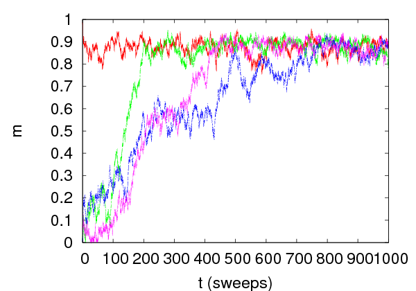


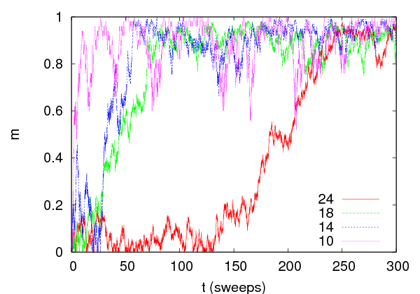


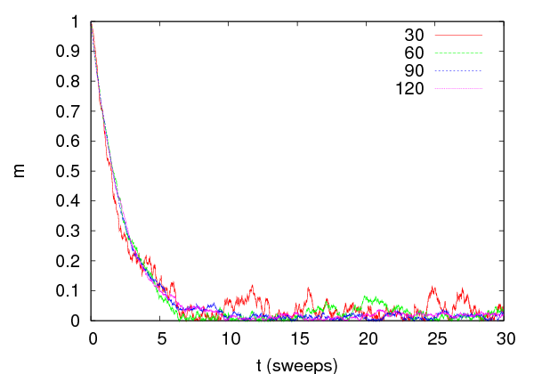


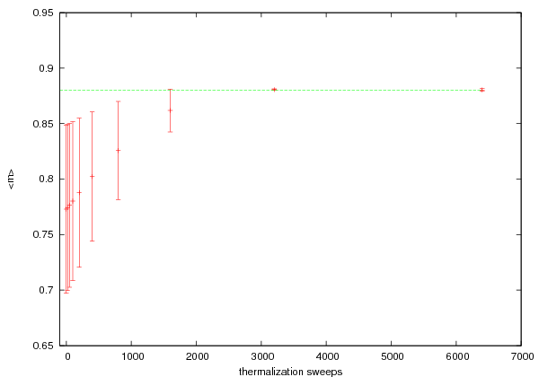


 and
and  initial measurements until the
expectation value of the magnetization stabilizes within the limits of its statistical
error.
 , correlations between configurations obtained after a few
sweeps remain strong. It is easy to understand why this is happening.
As the correlation length
  (
( (e.g. energy,
magnetization, etc) and let
  be its value after Monte Carlo “time”
  .
.  can be measured in sweeps or multiples of it. The autocorrelation function
  of
of  is
is

 is the average value over the configurations in the sample for
 . The normalization is such that
  .
.
 after time
  is strongly
correlated to the one at
  , then the product in the numerator in
(
 will be
positive. When the correlation is weak, the product will be positive and
negative the same number of times and
  will be almost zero. In the
case of anti-correlations
  is negative. Negative values of
  occur, but these are artifacts of the finite size of the sample and should be
rejected.
 drops exponentially

 is the time scale of decorrelation of the measurements of
  and it is called the
 . After time
  ,
,  has dropped to the
  of its initial value and then we say that we have an independent measurement
of
 . Therefore, if we have
  measurements, the number of independent
measurements of
  is
is 
 sweeps. If the cost
of measurement is not significant, then we usually measure more often, since there
is still statistical information even in slightly correlated configurations. An
accurate determination of
  is not easy since it requires measuring for
  .
.
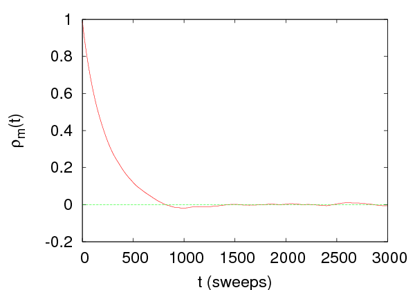


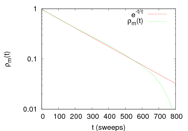


 ). We calculate the function
  and we see that a fit to equation
(
 sweeps. The calculation is performed on a
sample of
  measurements with 1 measurement/sweep. Therefore the number
of independent measurements is
  .
.
 . Its definition stems from equation (
 and
and  differ slightly due to systematic errors that come from the
corrections

 we observe a plateau in the plot of the value of
 which indicates convergence, and we take this as the estimator of
 . For even larger
  , finite sample effects enter in the sum that should be
discarded.
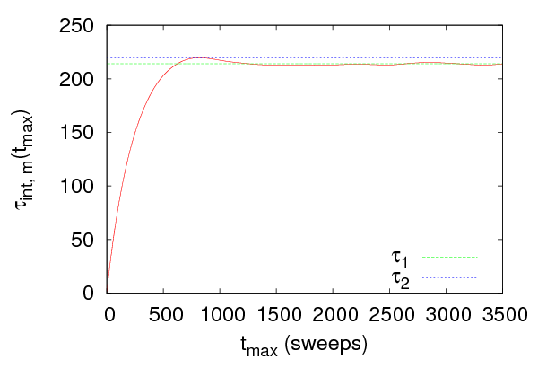


 sweeps, which
is somewhat smaller than the autocorrelation time that we calculated
using the exponential fit to the autocorrelation function. If we are
interested in the scaling properties of the autocorrelation time with the
size of the system
  or the temperature
  , then this difference is not
important
 is quicker since it involves no
fitting


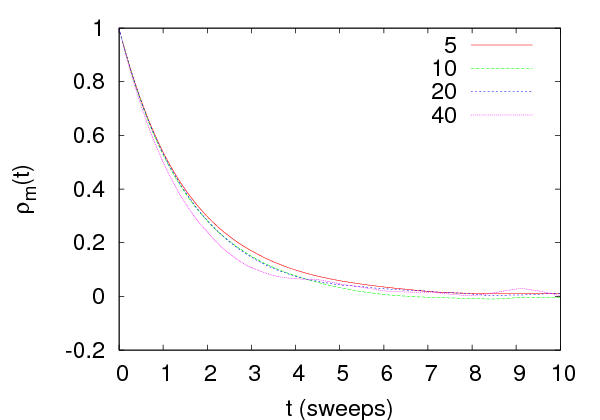


 . As we approach the critical region,
autocorrelation times increase. At the critical region we observe scaling of their
values with the system size, which means that for large
  we have that


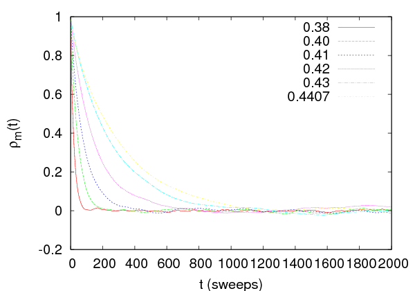

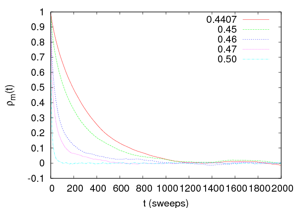


 measurements
 , their mean is an estimator of


 , then according to equation
 independent measurements. One can
show that in this case, the statistical error in the measurement of
  is
is
 , then we obtain equation (

 independent measurements (we
assumed that
  ). The above relation is consistent with our
assumption that measurements become independent after time
  .
.
 and
and  (or
(or  on each
configuration
  ). After these are calculated on the sample, the error
  is not a simple function of
  and
and  . This is because of the
correlation between the two quantities and the well known formula of
error propagation
  cannot be
applied.
 measurements, she can put them in
  “bins” and
each bin is to be taken as an independent measurement. This will be
true if the number of measurements per bin
  . If
. If 
 is average value of
  in the bin
  , then the error is given by
(
 (see
equation (
 . If
. If  is not a priori known we compute the error (
 . When the error is not increasing anymore and takes on
a constant value, then the calculation converges to the true statistical
error.
 bins which contain
  elements as
follows: The bin
  contains the part of the sample obtained after we
we
  -th bin of the binning method from the
full sample
  . The procedure is depicted in figure


 in each bin and we obtain
 . Then the statistical error in the measurement of
  is
is


 random samples as follows: We choose one of the
  measurements
with equal probability. We repeat
  times using the
  measurements - i.e. by putting the chosen measurements back to the sample. This
means that on the average
  of the sample will consist of the
same measurements. In each sample
  we calculate the average
values
  and from those


 is
is

 without an a priori knowledge of
  . For more details, the
reader is referred to the articles of Bradley Efron
  measurements
  ,
then we can use the following estimator for the autocorrelation function, given by
equation (

 is chosen so that
  .
.
 , the second one is
  and the third one is
  (equation (
 we do the following:
 . The
. The  stabilizes and
the
 is minimized
 of the fit can be read off from the output of the command
 . We stress that this is the
  doubles its minimum value, we find that
  .
.
 .
.

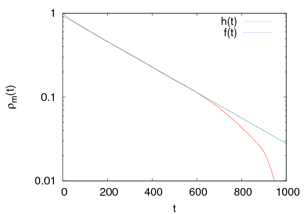


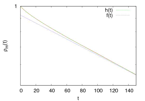
 . We find that the data for
the autocorrelation function fit perfectly to the function

 fit is excellent and the
result for the dominant autocorrelation time is
  . The
secondary autocorrelation times are
  ,
,  which are
considerably smaller that
  .
.
 and then
we use equation (
 ,
,  ,
,  and
and
 .
. lattice sites
(
 (-b 0.4407). It starts the simulation from a hot
configuration (
 and
and  with their errors using the program
  and their error by the factor
  in order to obtain
 .
.
 ,
,  and
measure the magnetization per site (
 measurements
using the commands:
 . The integrated autocorrelation time is found to be
 .
.
 . The application of equation
(
 . Using equation (
 .
The error of the magnetic susceptibility cannot be calculated this way.

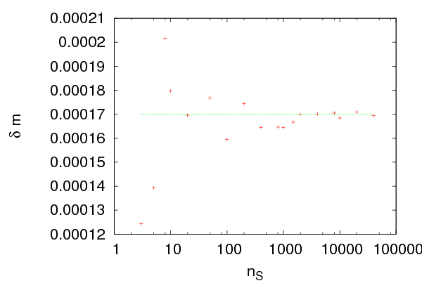


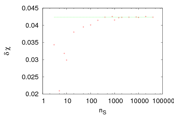


 so that the optimal number of samples is
be determined. Figure
  for quite small
number of samples. The analysis could have safely used
  . In the
case of the magnetic susceptibility, convergence is slower, but we can
still use
  . We obtain
  and
and  . The error
assumes independent measurements, something that is not true in our case.
We should use the correction factor
  which gives
  .
Therefore

 . The a priori knowledge
of
  is necessary in this calculation.
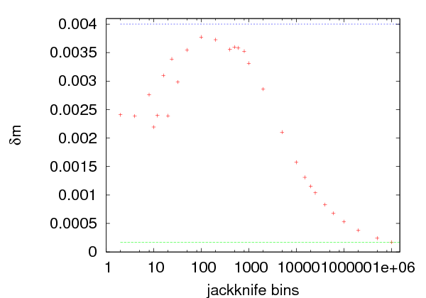


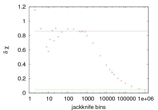


 . The errors are calculated for a variable number of bins
 . Figure
  the
samples consist of all the measurements except one. Then the error is equal to the
error calculated using the standard deviation formula and it is underestimated by
the factor
the
samples consist of all the measurements except one. Then the error is equal to the
error calculated using the standard deviation formula and it is underestimated by
the factor  . This is shown in figure
  . The effect of the autocorrelations
vanishes when we delete
  measurements from each bin. This
happens when
  . Of
course this an order of magnitude estimate and a careful study is necessary in
order to determine the correct value for
  . Figure
  to the value
  , which is quite close to
the value
  . We note that, by using a small number
 , we obtain an acceptable estimate, a rule of the thumb that can be
used for quick calculations.
 , where the
error converges to the value
  , in accordance with the previous
estimates. For
  the error converges to the underestimated error
 .
.
 ,
,  without calculating
  directly. The
data is split into
 . Each
jackknife bin contains
  data elements and we apply the bootstrap
method on this data, by taking
  samples of
  random data. Then
each jackknife bin gives a measurement on which we apply equation (
 and the true
error
  using one of the methods described above, we can calculate
  using
the relation
  . Therefore

 using all the methods described here, these relations can also
be used in order to check the analysis for self-consistency and see if they agree.
This is not always a trivial work since a system may have many autocorrelation
times which influence each observable in a different way (fast modes, slow
modes).

 on the temperature and
the size of the system. Take
  and
and 


 . Then take
  ,
, 


 . Repeat for the same values of
  for
for  and
and
 .
.
 . Repeat for
  .
Compare your results with
  and
and  .
.
 and
and  as a function
of
  (see figure
  and
and  as a
function of
  (see figure
  (see equation (
 for
for  and
and  at an interesting
range of temperatures. Use different initial configuration in order to
study the thermalization of the system as
  increases: Cold state with
spins parallel to
  , cold state with spins antiparallel to
  and hot
state. Study the dependence of the critical temperature separating the
ordered from the disordered state on the value of
  .
.
 has a
first order phase transition, i.e. a discontinuity in the value of the order
parameter which in our case is the magnetization as a function of
  . Near
a first order transition we observe the phenomenon of hysteresis. In order to
see it, set
  and
and  and
and

 using as an initial state the last
one coming from the previous step. Do 100 sweeps and calculate
 .
.
 .
Stop when
  .
.
 until
until  .
.
 until
until  .
. . What do you observe?
 sweeps per point. Plot the time series of
the magnetization and observe the transitions from the metastable
state to the stable one and backwards. Compute the histogram of
the values of the magnetization and determine which state is the
metastable in each case. How is the histogram changing as
  is
increased?
 instead of
  . Look into
chapter 13.1.2 of Newman and Barkema (esp. figure 13.4). Compute the
change in energy for each spin flip for the Metropolis step. Calculate the
maxima of the magnetic susceptibility and of the specific heat and see if
they are close to the expected critical temperature
  .
Note that even though
  is different than the corresponding value
on the square lattice, the critical exponents are the same due to
universality.
 to be the
 coordinate. Set
 and compute the energy, the
  , the specific heat, the
magnetic susceptibility
  and the
  .
.
 has a maximum in the region
  . Compute its value at this
temperature for
  . Show that
  does not diverge as
  ,
therefore
  does not show a phase transition.
 . What do you conclude? Compare the
behavior of
  for the antiferromagnetic Ising model with
  of the
ferromagnetic.
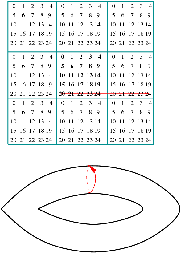

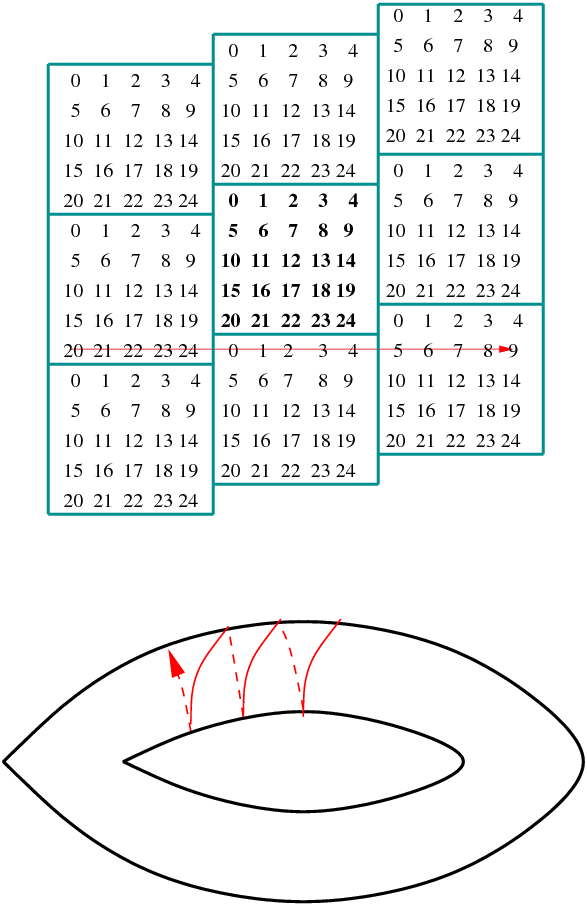





 , or equivalently as the reduced
temperature
 , calculated in
 , which are the same for all
systems in the same
  , when
  . Systems with the same long distance behavior, but which
could possibly differ microscopically, belong to the same
  these details become irrelevant and all these systems
have the same long distance behavior. Microscopic degrees of freedom of
systems in the same universality class can be quite different, as is the
case of the liquid/vapor phase transition at the triple point and the Ising
model.


 . For a finite
lattice, all observables are analytic since they are calculated from the
analytic
 given by equation (
 the
model behaves approximately as the infinite system. As
  and
and 
 and
and  , on the finite
lattice have a maximum for a
  for which we have
that

 , we have
that

 , therefore equations
(


 , but
they can also be evaluated at any temperature in the
  , but one can also use e.g.

 according
to (
 in this region, and we
obtain equation (
 . When
  we have the effect of critical
slowing down.
 is
concerned
 .
But the measurement of a local quantity, like
  , for a given number
of times requires no extra cost, since each configuration yields
  measurements
 is preferable, since it reduces
finite size effects. We see that, in the absence of critical slowing down, the cost of
measurement of
  is
is  .
.
 , making the large
  simulations
prohibitively expensive. For the Metropolis algorithm on the two dimensional
Ising model we have that
  ; and the problem is severe. Therefore, it is
important to invent new algorithms that beat critical slowing down. In the case of
the Ising model and similar spin systems, the solution is relatively easy. It is
special to the specific dynamics of spin systems and does not have a universal
application.
 . As we approach the critical temperature
  from the
disordered phase, the typical configurations are dominated by large clusters of
same spins. The Metropolis algorithm makes at most one spin flip per step and
the acceptance ratios for spins inside a cluster are small. For example, a spin with
four same neighboring spins can flip with probability
  ,
which is quite small. The spins that change more often are the ones with
more neighbors having opposite spins, therefore the largest activity is
observed at the boundaries of the large clusters. In order to obtain a
statistically independent configuration, we need to destroy and create
many clusters, something that happens very slowly using the Metropolis
algorithm who realizes this process mostly by moving the boundaries of the
clusters.
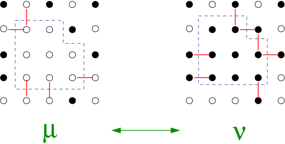
 , whereas large clusters
of size
  should dominate for
  .
.
 . If
. If  is
properly chosen, the detailed balance condition (
 , the cluster is enclosed by the dashed line. The new state
  is obtained
by flipping all the spins in the cluster, leaving the rest of the spins to be the
same.
 will yield equation (
 and
and
 . This can be seen in the simple example of figure
  of the new state
  and the acceptance ratio
 , so that

 !
!
 is the probability of constructing a
particular cluster and can be split in three factors:


 is the
probability to include all cluster members found in the
  , the corresponding term is exactly the same since
the two clusters are exactly the same (the only differ by the value of the
spin)!

 is the probability to include a nearest neighbor of same spin to
the cluster, the probability of saying “no” is
  . Assume that we have
  “bonds”
 , and that we have
  such bonds in the state
  . In figure
  and
and  . Therefore, the probability to stop the cluster in
the state
  is to say “no”
  times, which happens with probability
 :
:

 stops at the same boundary with
probability


 decreases the energy by 2 and each bond destroyed increases the energy
by 2:

![m− nA (μ → ν ) −2β(m −n) A(μ → ν) [ 2β ]n−m
(1 − Padd) ----------= e ⇒ ----------= e (1 − Padd) .
A (ν → μ ) A(ν → μ)](main_latex5373x.png)


 given by (
 .
This is the first new member of the cluster
 .
The original spin is not a “new member” anymore
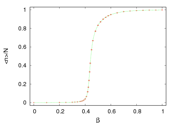


 depends on the temperature
  . It is quite small for
 and almost 1 for
  . Therefore, in the first case the algorithm
favors very small clusters (they are of size 1 for
  ) and in the second
case it favors large clusters. In the high temperature regime, we have
almost random spin flips, like in the Metropolis algorithm. In the low
temperature regime, we have large probability of flipping the dominant cluster of
the lattice. This is clearly seen in figure
  is plotted as a function of the
temperature. For small
  ,
,  whereas for large
  ,
,  .
.
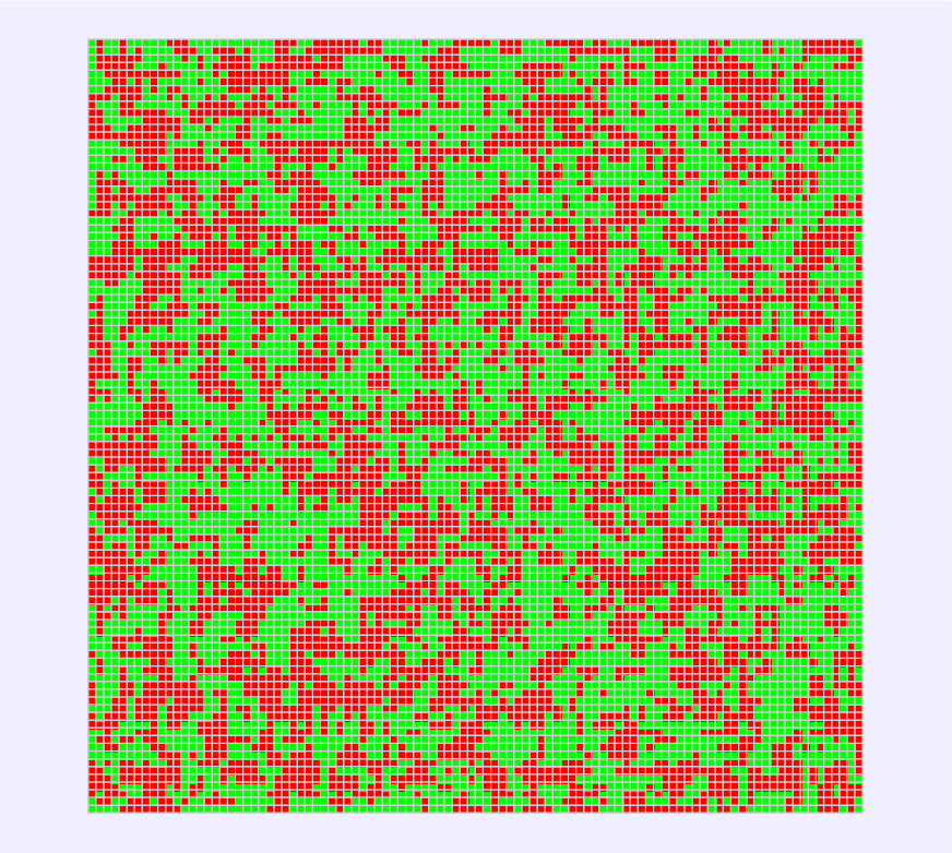
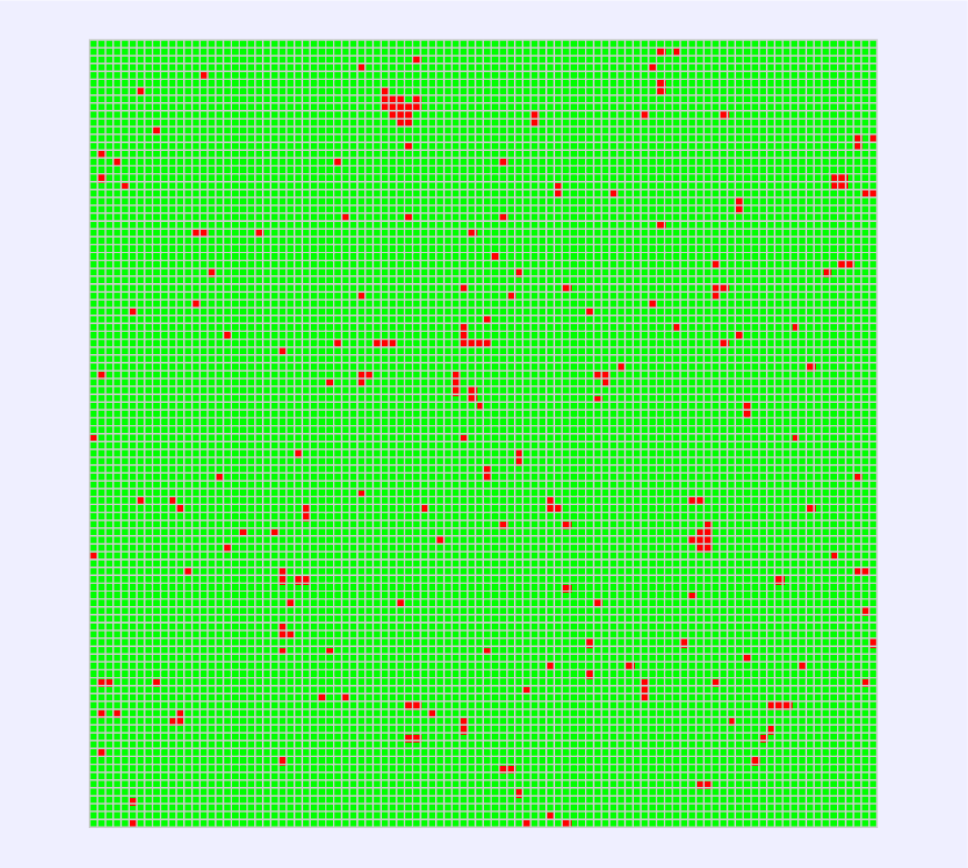


 , most of the time the algorithm chooses a lattice site
randomly and constructs a small cluster around it and flips its spins. The
Metropolis algorithm picks a lattice site randomly and flips it most of the
times. In both cases, the two algorithms function almost the same way and
construct the high temperature disordered spin configurations. For large
  ,
a typical spin configuration is a “frozen” one: A large cluster of same
spins with a few isolated thermal fluctuations of different spins. Most of
the times, the Wolff algorithm picks a seed in the dominant cluster and
the new cluster is almost the same as the dominant cluster: Most of its
sites are included with few ones excluded, which upon flipping of the
spins, they will form the new thermal fluctuations. After the flips, the old
thermal fluctuations have the same spin as the dominant cluster and they
become part of the new dominant cluster. The Metropolis algorithm picks
lattice sites randomly: When they belong to the dominant cluster they are
seldomly flipped, whereas the thermal fluctuations are flipped most of the
time. Both algorithms function similarly and have the same efficiency.
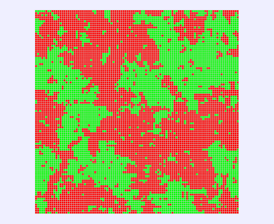
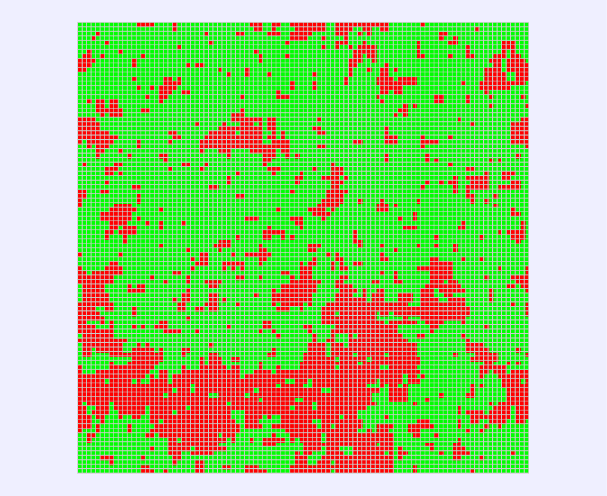


 ). In
contrast, the Metropolis algorithm modifies clusters by slowly moving their
boundaries and large clusters are destroyed/created very slowly. Autocorrelation
times are expected to reduce drastically when using the Wolff algorithm in the
critical region.
 ) we have
that

 . In the end, the lattice will be divided in
  Wolff
Wolff sites, whose spin is
  . Choose a lattice site
randomly and flip the spins of the cluster it belongs to. Destroy the bonds and repeat the
process

 are equally probable due to the symmetry of the model,
therefore the first term vanishes. Since
  , we obtain

 is
is


 we have that


 .
.

 . The new members of the
cluster are pushed into the stack
 (it
has been set in
  ), then we add
  is defined in
  ,
,  , by constructing 5000 clusters, starting from a
hot configuration and writing the data to the file
  , we have to
perform simulations for many values of
  . Then, we want to study the finite
size properties and extrapolate the results to the thermodynamic limit,
by repeating the process for several values of
  . The process is long
and ... boring. Moreover, a bored researcher makes mistakes and several
bugs can enter into her calculations. Laziness is a virtue in this case and
it is worth the trouble and the time investment in order to learn some
techniques that will make our life easier, our work more efficient, and
our results more reliable. Shell scripting can be used in order to code
repeated tasks of the command line. In its simplest form, it is just a series of
commands written into a text file. Such an example can be found in the file
 (
( –
–  . Each
simulation starts from the configuration stored in the file
  ,
,  , ... ,
  , each time with
  and
and
 .
.
 and the
magnetization per site
  with their errors can be calculated by the
jackknife program, which can be found in the file
  can be
calculated using the command:
 . The condition
 and its error and then the fluctuations
  and their error.
The latter must be multiplied by
  , in order to obtain the specific
heat
  and its error according to (
 and/or
  , by editing the values of the variables
  and
and  .
.
 .
The result is
 and
and  .
.
 :
:
 .
.
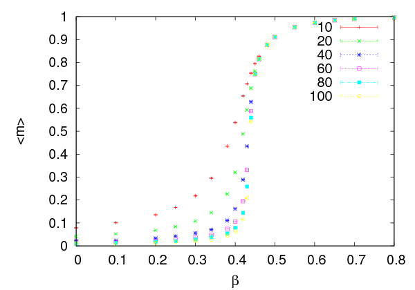


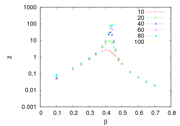


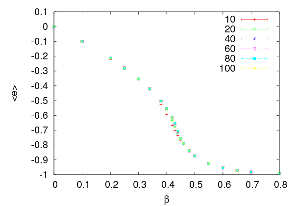

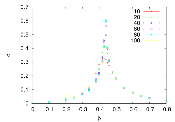


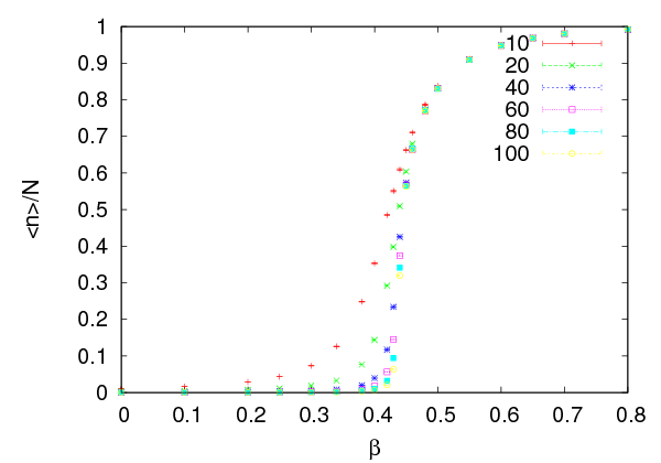

 .
.


 –dependent unit of time equal to one Wolff
cluster update. We use the notation
  when the autocorrelation time of
  is
measured in Wolf cluster updates, and
  when using the definition (
 and
and  at
at
 using the Wolff algorithm. We construct
  Wolff clusters. The
results are written to files with names
  sweeps. The results are
written to files with names
  :
:
 sweeps for thermalization. The results are
written to files whose names have file extension
  is fitted to (


 where
where  is the dynamic exponent
 can be calculated by the
  is calculated for the Wolff algorithm in Wolff steps and Wolff
sweeps. The results are


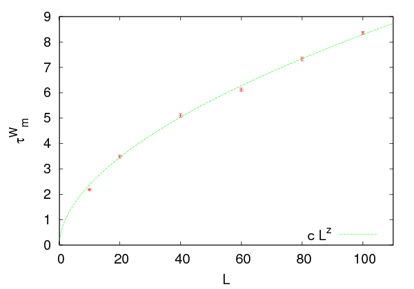


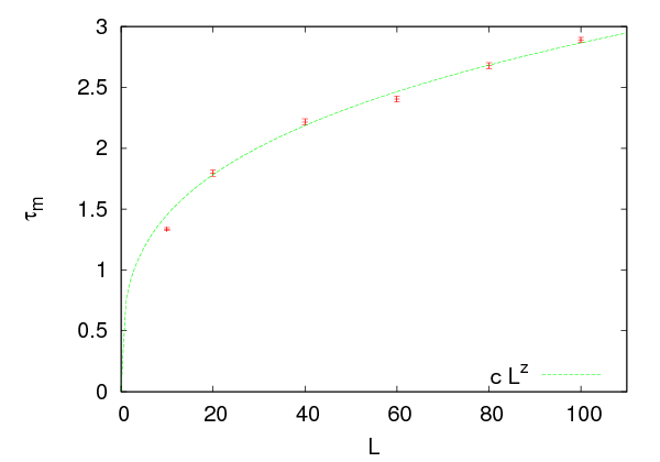


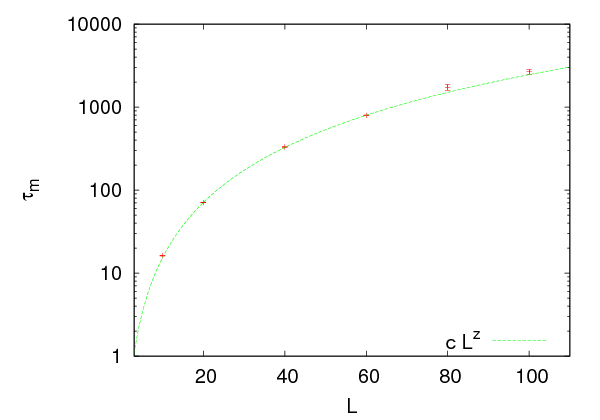


 reported in the
bibliography are
  ,
,  and
and  respectively
  , (
, ( ,
and (
 and using
  , valid in the critical region, we
obtain

 ,
,  and
and  . Therefore

 ,
,  , we obtain


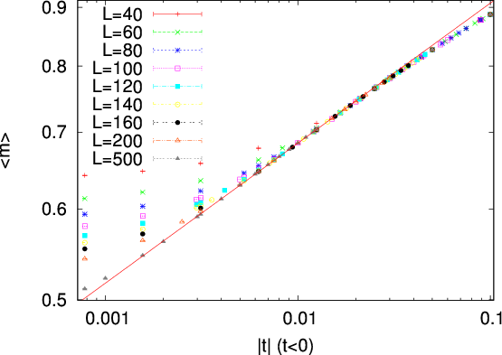


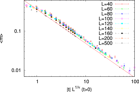


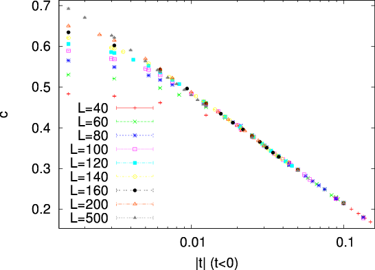


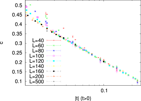


 ,
,  and
and  . The result is that, although
using them it is possible to compute correct results, these relations are not the best
choice
 and large
  . The results depend strongly on the choice of range of the data included
in the fits. The systematic errors are large and the results in some cases plain
wrong
 ,
,  ,
,  ,
,  ,
,  ,
,  ,
,  ,
,
 and
and  . The temperatures chosen correspond to small enough
  in order
to observe scaling. For the values of
  used in the simulations, see the shell
scripts in the accompanying software.
 from the relation (
 , we fit the data for
  for an appropriate range of
  to
the function
  , which has two fitting parameters,
  and
and  . We
determine the range of
  where
where  gives a linear plot in a log–log
scale
 , we observe deviations from the linear behavior and for very small
 we observe finite size effects when
  . As
. As  increases, finite size effects
decrease, and the data get closer to the asymptotic behavior
  for even
smaller
  . The results are more clear for
  , because for
  the
fluctuations near the pseudocritical temperature
  are larger and the
finite size effects are larger.
 for all the measured values of
 . The errors reported are the statistical errors of the fits, which are smaller
than the systematic errors coming from the choice or range of
  of the data
included in the fits. One has to vary this range as long as the
  dof of the fit
remains acceptable, and the resulting variation in the values of the parameters has
to be included in the estimate of the error. Sometimes, this method gives an
overestimated error, and it is a matter or experience to decide which parameter
values to include in the estimate. For example, figures
  for
increasing
  . As
. As  increases, the points approach the asymptotic curve
even closer. Even though for fixed
  one obtains acceptable power fits
over a larger range of
  , by studying the large
  convergence, we can
determine the scaling region with higher accuracy. Another point to consider is
whether the parameters of the fits have reasonable values. For example, even
though the value of
  is unknown, it is reasonable to expect that its
value is of order
  . By taking all these remarks into consideration we
obtain


 using relation (
 or
or  . In the thermodynamic limit, the magnetization is everywhere zero for
all
  . For a finite lattice
  , and it is reasonable to expect a scaling
of the form

 is defined so that

 and
and  shown in table

 .
.
 needs special care. The expected
value is
  . This does not imply that
  const. but that

 plot. We see that the second choice leads to a
better linear plot than the first one. A careful study will compute the quality of
the fits and choose the better model this way. This is left as an exercise for the
reader.
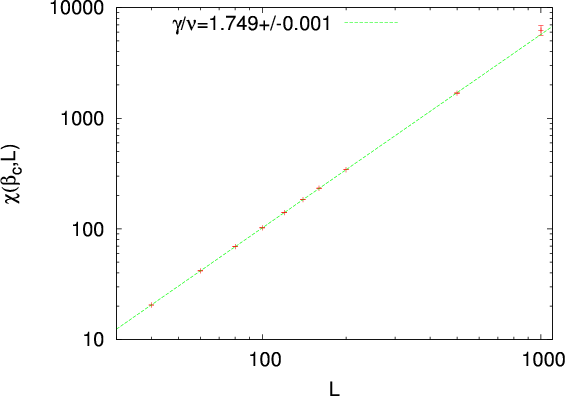


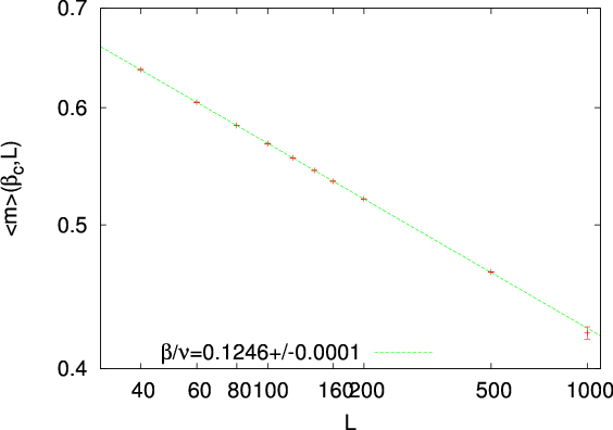


 ,
,  and
and
 with increasing system size
  . This is called “finite size
scaling”.
 given by equation (
 for increasing values of
  .
We fit the results
  to the function
  and calculate the fitting
parameters
  and
and  . Then, we compare the computed value of
  to
the expected value of
  . In this procedure we have to
decide which values of
  should be included in the fits. The most obvious
criterion is to obtain reasonable
  and that the error in
  and
and
 be small. This is not enough: Table
  , if we consider different fit ranges. These
variations give an estimate of the systematic error which enters in the
calculation. Problem
 given by equation (
 at the critical temperature and repeat the
same analysis. The result is

 . But the expected value
  leads, in analogy with equation (
 and appreciate the difficulties
that arise in this study. By increasing the statistics, and by measuring for
larger
  , the data in table


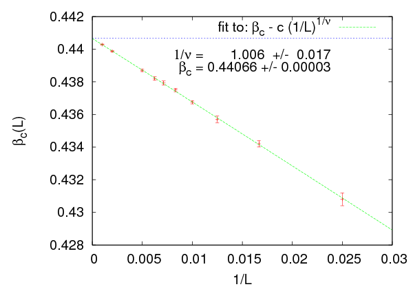


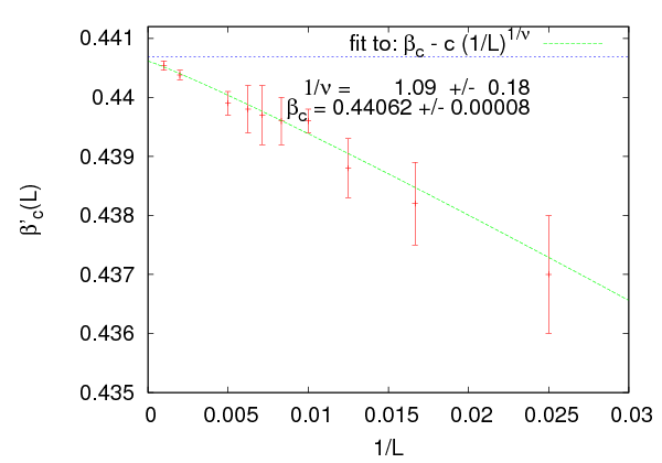


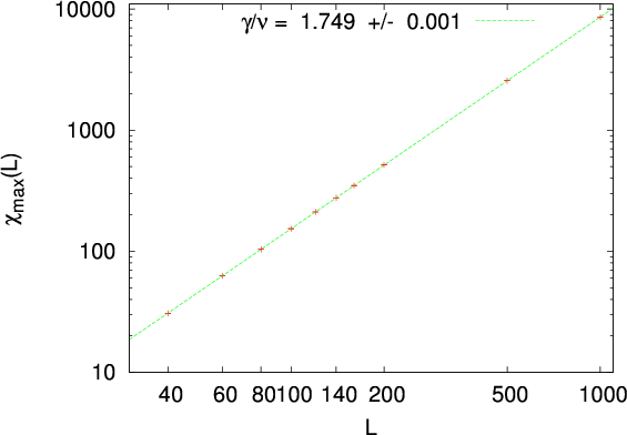


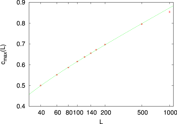


 and
and  in the critical region.
In the calculations we used the exact value of the critical temperature
 . When
  is not known, the analysis becomes harder and
its computation contributes to the total error in the value of the critical
exponents. When doing finite size scaling using the scaling relations (
 . What should we do
when
  is not a priori known? A good choice is to use the pseudocritical
temperature
  , the temperature where the fluctuations of the order
parameter
  are at their maximum. Otherwise, we can compute
  according to the discussion in this section and use the computed
  in the finite
size scaling analysis.
 limit, even though the
finite size effects are different. In fact any value of
  in the critical region can be
used for this calculation. The reason is that as we approach the critical region for
given
  , the correlation length becomes
  and finite size effects become
important. This is the behavior that characterizes the
  system. The pseudocritical region becomes narrower as
  becomes
larger. Any value of
  in this region will give us observables that scale at large
 , but the best choice is

 .
.
 in not unique. One could use, for example, the
maximum of the specific heat

 . Of course

 and both choices will yield the same results for large
  . The speed of
convergence and the errors involved in the calculation of the pseudocritical
temperatures are different in each case and there is a preferred choice, which in
our case is
  .
.
 . When we are in the pseudocritical region we have that
 , therefore (
 we determine the pseudocritical region and
we calculate
  and the corresponding maximum value
  . In
order to do that, we should take many measurements around
  . We
have to be very careful in determining the autocorrelation time (which
increases as
  ), so that we can control the number of independent
measurements and the thermalization of the system. We use the relation
(
 , and from the calculated parameters
 and
and  we compute
  ,
,  . In cases where one of the
parameters
  ,
,  is known independently, then it is kept constant during the
fit.

 and
and
 .
.
 and the
maximum values of the specific heat
  . The results are shown in figure
 we can calculate the
exponent
  . Their values are shown in table
  ,
according to the asymptotic relation (
 and
and  being fitting
parameters. We find very good scaling, therefore our data are in the asymptotic
region. The result is

 .
.
 .
Since
  , the form of the asymptotic behavior is given by (
 and it is possible
that the discrepancy is due to finite size effects. We add terms that are subleading
in
  and find that the fit to the function
  is very
good
 , the quality of the fit
is poor and the result for
  is consistent with zero. The results are shown in
figure
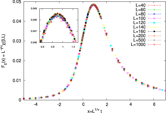


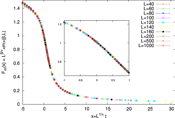


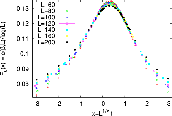


 . As we approach the critical point,
  diverges as
  , and we obtain
universal behavior for all systems in the same universality class. If we consider the
magnetic susceptibility
  , its values depend both on the temperature
  ,
the size of the system
  and of course on the details of the system’s degrees of
freedom and their dynamics. Universality leads to the
  . For the finite system in the pseudocritical region, finite
size effects suppress the fluctuations when
  . The length scales
that determine the dominant scaling behavior
  are
are  and
and  ,
therefore the
  is the only independent variable in
the scaling functions. In order to obtain the scaling relation
  ,
valid for the infinite system, we only need to assume that for the finite
system
 is a function of

 (
( ) the magnetic susceptibility takes values very
close to those of the infinite system, and (
 . As
. As  ,
finite size effects enter and (
 . The latter is
nothing but (
 describes
how the magnetic susceptibility deviates from scaling due to finite size
effects.
 can be calculated using the measurements coming from
the Monte Carlo simulation. Since the correlation length is not directly calculated,
but appears indirectly in the measurements, we define the dimensionless
variable

 since
since . We define
  so that (
 are determined by the
relations (
 , equation (
 and we obtain
  From the definition
 we obtain
  and we confirm the
scaling property of the magnetic susceptibility in the thermodynamic limit
 . Therefore

 , (
, ( .
Then we obtain
  Therefore, we
confirm that, when finite size effects are dominant (
 ), we have that
 . Therefore


 are measurements for temperatures in the pseudocritical
region for several values of
  . When equation (
 independently of
the size
  ! Of course deviations due to finite size effects are expected,
especially when
  is small. But, as we will see, convergence is quite
fast.
 , the
exponent
  and the ratio
  simultaneously! In order to check (
 , for which it is necessary to
know
  (
( ) and the exponent
  . For the calculation of
 it is necessary to know
  that appears on the right hand side of
(
 ,
,  and
and  and this way we obtain an accurate method for their
calculation.
 . Using
  ,
,  ,
,  and
and  , we calculate the scaling variable
 . Using
  and
and  , we calculate
 and plot the points
  near the critical region
 . Then we vary
  until the curves for different
  collapse onto
each other. The optimal collapse determines
  .
.
 for different
  is the most efficient
method for studying scaling in the critical region. Figure
  for the known values of the parameters
 . Small variations of the parameters lead to a sharp change
of the quality of the collapse. We can make a quick and dirty estimate of the
accuracy of the method by varying


 . The results are shown in figures
  whereas the ones starting with
  . The program can
be found in the file
  separated
from another by one or more spaces. The variables
  ,
,  and
and  that will be used in the scaling relation (
 (the index
 and its
error
  ). For
  , the
, the  bins and work
independently on each set of data. Each bin will give an optimal set of
parameters
  which will be assumed to be an independent
measurement. The errors can be calculated using equation (
 ).
).
 similar to the one used in data fitting, as discussed in appendix
 should increase. Assume that our measurements consist of
  sets of
measurements for
  . After setting the parameters
 and an interval
 ![Δx ≡ [x ,x ]
min max](main_latex5932x.png) , we calculate the data sets
, we calculate the data sets
 , for all
  , using our measurements.
The data sets consist of
  points of the data for
  , for which
the
  are in the interval
  . For each point
  , we calculate the
scaling function
  , which depends on the
chosen parameters
  and the lattice size
  . Then, we have to choose
an interpolation method, which will define the interpolation
 in a data set has a well defined distance
from every other data set
  (
( and
and  ), which is defined by the
distance from the interpolating function of the other sets. This is equal
to
 . We define the quantity
 is the number of terms in the sum. The normalization
constant
  is used, because this is the number of pairs of curves in the
sum. Each term is weighted by its error
  , so that points with
small error have a larger contribution than points with large error. This is
the definition used in
  depends on the parameters
  and the interval
  . Initially,
we keep
  fixed and perform a minimization with respect to the parameters
 . The minimum is given by the values
  and these values are the
estimators that we are looking for. In order to calculate the errors
  we can bin
our data according to the discussion on page
  distribution of the measurements, and if the minimum
  , then the
intervals of the parameter values that keep
  give an estimate of the errors
in the parameters.
 . Usually
  so that
 ![Δx = [xmax − δx, xmax + δx]](main_latex5967x.png) . If
. If
 is larger than it should, then
  is large and we don’t have good
scaling. If it is too small, then the errors
  will be large. By taking the limit
 , we calculate
  by studying the convergence of
  to stable, optimal
with respect to error, values (see figure 8.7, page 238 in


 corresponds to the Gaussian distribution, whereas the value
  corresponds to two Gaussian distributions of small width around two symmetric
values
  (see problems
  are small,
therefore the calculation of
  gives an accurate measurement of
the critical temperature
  . The curves
  intersect at the point
(
 ,
,  ) for different
  and this point gives a very good estimate of
 .
.


 . The intersection of the
curves in the figure at a single point (
 ,
,  ) is impressively accurate. Table
 systematically by computing the critical
temperature from the intersection of the curves
  for three values of
  .
By taking into account all the measurements for
  –
–  the computed
result is

 ,
,
 . Notice that, in the calculation of
  the systematic error
due to finite size effects decreases with increasing
  , whereas the statistical error
increases due to the increase of the slope of the curves
  near the point
 . But the accuracy of the calculation of
  turns out to be better with
increasing
  .
.
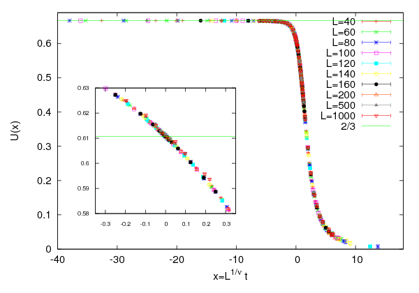


 and
and  . From equation (
 scales as

 , we obtain
 , which is consistent with the result (
 , can be
hard in the general case. Therefore it is desirable to cross check results using
several observables which have known scaling behavior. We discuss some of them
below
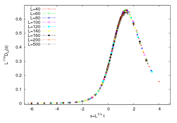


 defines a pseudocritical region
around its maximum. The scaling of the maximum as well as the scaling of its
position can be used in order to compute
  , as we did in figures


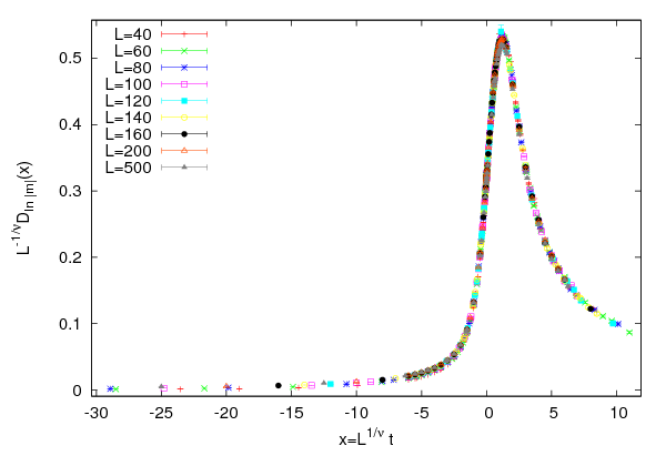


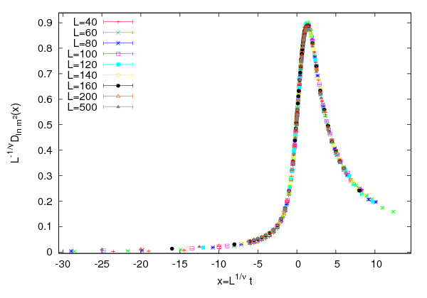


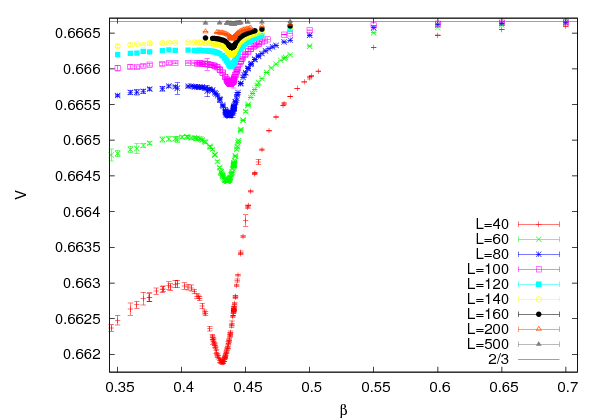


 ,
whereas for a first order phase transition, we obtain a non trivial value. Therefore,
this parameter can be used in order to determine whereas a system undergoes a
first order phase transition. This is confirmed in figure
  converge to the critical temperature according to (
 and its derivatives. For more
details, the reader is referred to
  are trivial in two cases: When the magnetization follows a
Gaussian distribution, which is true in the high temperature, disordered phase, we
have that
  . When we are in the low temperature, ordered phase, we have
that
  . The proof is easy and it is left as an exercise (see problems
  of a continuum phase transition is approached, the system exhibits scaling
properties due to the diverging correlation length
  . If we approach
  from the
high temperature phase, then we expect that the distribution function of the
magnetization per site
  (not its absolute value) is approximately of the
form


 . We have
temporarily assumed that the system is defined on a
  –dimensional hypercubic
lattice of edge
  .
.
 scales according to the relation


 ,
,  , is the correlation
length
  , in such a way that
  . Equation (
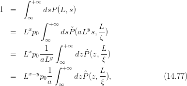
 . For the left hand side to be equal to one, we must have
that
  ,
,

 .
.  ,
,  and
and  is a constant
independent of
  and
and  . Finally, we obtain

 are
are 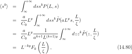
 . When we
  and
and  , the correlation length
  diverges in such a way that
  .
In the region
  (
( ) we have that
  , and by using the
relations


 and
and  ,
which are universal constants (i.e. they are the same within a universality class)
and they are defined from equation (
 on the right and left hand
sides
 -scaling, we substitute the above equations to (
 , and we obtain


 ,
,


 . From equation (
 keeping
  finite, and the
fluctuations get suppressed, rendering the functions
  finite. Therefore, we
obtain
 at the critical temperature turned out to be
almost independent of the system size
  .
.  is found to depend on the
boundary conditions and on the anisotropy of the interaction. For the Ising model
on the square lattice we have that

 is the dimensionless correlation length in the thermodynamic
limit and
  is the scaling factor
 is the reduced temperature and
  is the external magnetic
field
 and
and  give the change in the coupling constants
  and
and
 under the change in length scale in order that the equation remains
valid.
 times we obtain

 ,
,  , keeping the product
  fixed, we
obtain
 and
and  and the
critical exponent


 ,
,  , keeping the product
  , the left
hand side will give a finite value, e.g.
  whereas the right hand side will
give

 , and by comparing to the known relation (
 , we obtain


 whenever we neglect terms that are not related to the
scaling properties of a function.
 , we obtain the
specific heat
 is nothing but the critical exponent of the
specific heat defined in equation (

 we obtain the
magnetic susceptibility

 , we obtain


 (the volume is
  ,
,  is the number of
dimensions), where
  is the (dimensionless) number of lattice sites and
  is the
lattice constant. We consider the limit
  and
and  , so that
 -scale


 ,
,  and
and 

 (approach of the critical point), the above relation becomes

 as in the previous section we
obtain
 ,
, 
 .
.
 where
where  ,
which yields the known relation
  .
.
 is comparable to
  , finite size effects dominate. The large
fluctuations are suppressed and the magnetic susceptibility has a maximum at
a crossover (pseudocritical) temperature
  , where
 . The last relation holds because
  by assumption. We
obtain


 is analytic in its
argument
  , since for a finite system
  is an analytic function of the
temperature
 and
and  , therefore
  )
)


 . Near the
pseudocritical point

 we have that

 (equation (
 . This
increases the pseudocritical temperature
  (
(
 in (
in ( (
(
 in (
in ( (
(
 in (
in ( depends on the boundary conditions and the geometry
of the lattice.


 for
small
  . Then, we see that

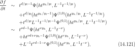
 . The term
proportional to
  vanishes when we set
  . In the pseudocritical region,
where
  , the first and third term are of the same order in
  and we
obtain


 ,
,  . The relation

 coming from the two point correlation function
 .
.


 for the Metropolis algorithm
as a function of the temperature for
  ,
,  ,
,  . Compute
the average size
  of the Wolff clusters at the same values of the
temperatures. Then calculate the number of Wolff clusters that are
equivalent to a Metropolis sweep. Make the plots of all of your results
and connect the points corresponding to the same
  .
.  ,
,  ,
,
 ,
,  ,
,  ,
,  .
.
 ,
,  ,
,
 ,
,  ,
,  ,
,  . Recalculate the dynamic exponent
  using
your data.
 ,
,  ,
,  ,
,  .
Recalculate the dynamic exponent
  using your data.

 , where
  is the average acceptance
ratio of the Metropolis algorithm. This changes the unit of time to
 .
.
 ,
,  ,
,
 ,
,  ,
,  . Choose appropriate values of
  , so that you will be
able to determine the magnetic susceptibility and the specific heat with
an accuracy comparable to the one shown in table
  and
and  by
computing the
  according to the discussion in appendix
  ,
, and
and  . Use the values in this table in order to make the
fits which give the exponents
  ,
,  and
and  as described in the
text. For the exponent
  , try fitting to a power and a logarithm
and compare the results according to the discussion in the text.


 ,
,
 ,
,  ,
,  and
and  . Make the appropriate fits in order to
calculate the exponents
  ,
,  ,
,  and the critical temperature
  as described in the text. For the exponent
  , try fitting to a power and a
logarithm and compare the results according to the discussion in the
text.
 . Vary each parameter separately, so that the collapse becomes
not satisfactory and use its variation as an estimate of its error.
Determine the range in
  that gives satisfactory collapse of the
curves. Repeat your calculation by performing measurements for
 , and using the data for
  . Compare the
new results with the previous ones and comment on the finite size
effects.
 we have that

 . Using this relation
calculate the derivative of the Binder cumulant
  and prove equation
(
 in order to
calculate the critical exponent
  according to the analysis shown in
figures
  we have that
 and
and  . Conclude that
  .
.

 . Show that
  and
and  .
Interpret your results, i.e. the meaning of each expectation value. Show
that for
  we obtain
  . Convince yourself that the
approximation used concerns the system in the low temperature
phase.
 as a function of
  ,
,  ,
,  and
and  . Apply finite size scaling arguments and prove equation (
 ,
,  in order to prove
the other relations in (
 ,
,  dof,
dof,  ,
,  ,
,  ,
,  ,
,  ,
,  ,
,  ,
,  ,
,  ,
,  ,
,  ,
,  ,
,  dof,
dof,  symmetry,
  ,
,  cycles,